
The picture classification structure is convenient for training and testing
1. Use convolution for complex images
#@title Licensed under the Apache License, Version 2.0 (the "License");
# you may not use this file except in compliance with the License.
# You may obtain a copy of the License at
#
# https://www.apache.org/licenses/LICENSE-2.0
#
# Unless required by applicable law or agreed to in writing, software
# distributed under the License is distributed on an "AS IS" BASIS,
# WITHOUT WARRANTIES OR CONDITIONS OF ANY KIND, either express or implied.
# See the License for the specific language governing permissions and
# limitations under the License.
In the previous experiment, you used the Fashion MNIST dataset to train the image classifier. In this case, your image is 28x28 with the theme centered. In this experiment, you will take it to a new level and train to recognize the features in the image, in which the subject can be located anywhere in the image!
You will do this by building a horse or man classifier that tells you whether a given image contains a horse or man, where the network is trained to identify features that determine which is which.
In the case of Fashion MNIST, the data is built into TensorFlow through Keras. In this case, the data is not so, so you must process it before you can train.
First, let's download the data:
!wget --no-check-certificate \
    https://storage.googleapis.com/laurencemoroney-blog.appspot.com/horse-or-human.zip \
    -O /tmp/horse-or-human.zip

!wget --no-check-certificate \
    https://storage.googleapis.com/laurencemoroney-blog.appspot.com/validation-horse-or-human.zip \
    -O /tmp/validation-horse-or-human.zip
--2021-09-08 23:03:26--  https://storage.googleapis.com/laurencemoroney-blog.appspot.com/horse-or-human.zip
Resolving storage.googleapis.com (storage.googleapis.com)... 209.85.147.128, 142.250.125.128, 142.250.136.128, ...
Connecting to storage.googleapis.com (storage.googleapis.com)|209.85.147.128|:443... connected.
HTTP request sent, awaiting response... 200 OK
Length: 149574867 (143M) [application/zip]
Saving to: '/tmp/horse-or-human.zip'

/tmp/horse-or-human 100%[===================>] 142.65M   139MB/s    in 1.0s

2021-09-08 23:03:27 (139 MB/s) - '/tmp/horse-or-human.zip' saved [149574867/149574867]

--2021-09-08 23:03:27--  https://storage.googleapis.com/laurencemoroney-blog.appspot.com/validation-horse-or-human.zip
Resolving storage.googleapis.com (storage.googleapis.com)... 74.125.124.128, 172.217.212.128, 142.250.152.128, ...
Connecting to storage.googleapis.com (storage.googleapis.com)|74.125.124.128|:443... connected.
HTTP request sent, awaiting response... 200 OK
Length: 11480187 (11M) [application/zip]
Saving to: '/tmp/validation-horse-or-human.zip'

/tmp/validation-hor 100%[===================>]  10.95M  32.0MB/s    in 0.3s

2021-09-08 23:03:28 (32.0 MB/s) - '/tmp/validation-horse-or-human.zip' saved [11480187/11480187]
The following python code will use the OS library to use the operating system library so that you can access the file system and the zipfile library so that you can decompress the data.
import os
import zipfile

local_zip = '/tmp/horse-or-human.zip'
zip_ref = zipfile.ZipFile(local_zip, 'r')
zip_ref.extractall('/tmp/horse-or-human')
local_zip = '/tmp/validation-horse-or-human.zip'
zip_ref = zipfile.ZipFile(local_zip, 'r')
zip_ref.extractall('/tmp/validation-horse-or-human')
zip_ref.close()
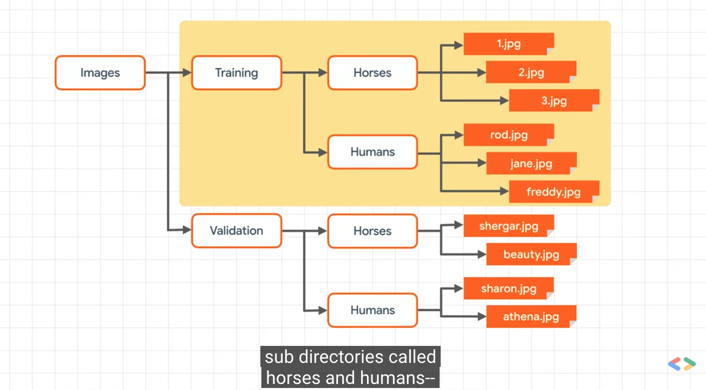
The contents of. zip are extracted into the base directory / TMP / horse or human, which in turn contains the horses and humans subdirectories, respectively.
In short: the training set is used to tell the neural network model "this is what a horse looks like", "this is what a man looks like" and other data.
One thing to note in this example is that we don't explicitly mark the image as a horse or man. If you remember the previous fashion example, we have marked "this is 1", "this is 7", etc.
You'll see later that something called an ImageGenerator is used -- it's encoded to read images from a subdirectory and automatically mark them from the name of that subdirectory. So, for example, you will have a "training" directory that contains a "horses" directory and a "humans" directory. The ImageGenerator marks the image appropriately for you, reducing the encoding steps.
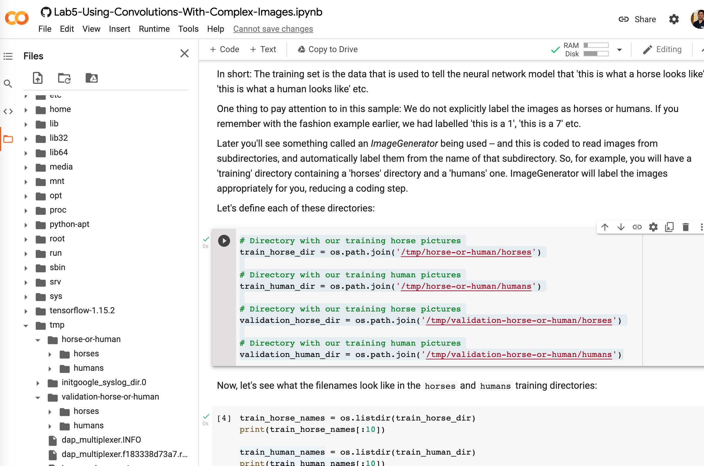
Let's define each directory:
# Directory with our training horse pictures
train_horse_dir = os.path.join('/tmp/horse-or-human/horses')

# Directory with our training human pictures
train_human_dir = os.path.join('/tmp/horse-or-human/humans')

# Directory with our training horse pictures
validation_horse_dir = os.path.join('/tmp/validation-horse-or-human/horses')

# Directory with our training human pictures
validation_human_dir = os.path.join('/tmp/validation-horse-or-human/humans')
Now let's look at the file names in the horses and human training directories:
train_horse_names = os.listdir(train_horse_dir)
print(train_horse_names[:10])

train_human_names = os.listdir(train_human_dir)
print(train_human_names[:10])
['horse42-9.png', 'horse15-4.png', 'horse43-0.png', 'horse40-1.png', 'horse16-0.png', 'horse15-5.png', 'horse09-0.png', 'horse02-7.png', 'horse47-0.png', 'horse32-7.png']
['human02-27.png', 'human14-25.png', 'human16-25.png', 'human09-04.png', 'human06-21.png', 'human05-29.png', 'human10-01.png', 'human08-13.png', 'human05-18.png', 'human17-18.png']
Let's find the total number of horse and man images in the catalog:
print('total training horse images:', len(os.listdir(train_horse_dir)))
print('total training human images:', len(os.listdir(train_human_dir)))
total training horse images: 500
total training human images: 527
Now let's look at some pictures to better understand their appearance. First, configure the matplot parameter:
%matplotlib inline

import matplotlib.pyplot as plt
import matplotlib.image as mpimg

# Parameters for our graph; we'll output images in a 4x4 configuration
nrows = 4
ncols = 4

# Index for iterating over images
pic_index = 0
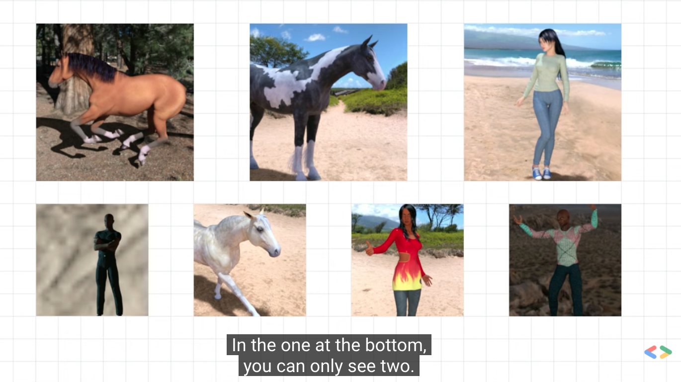
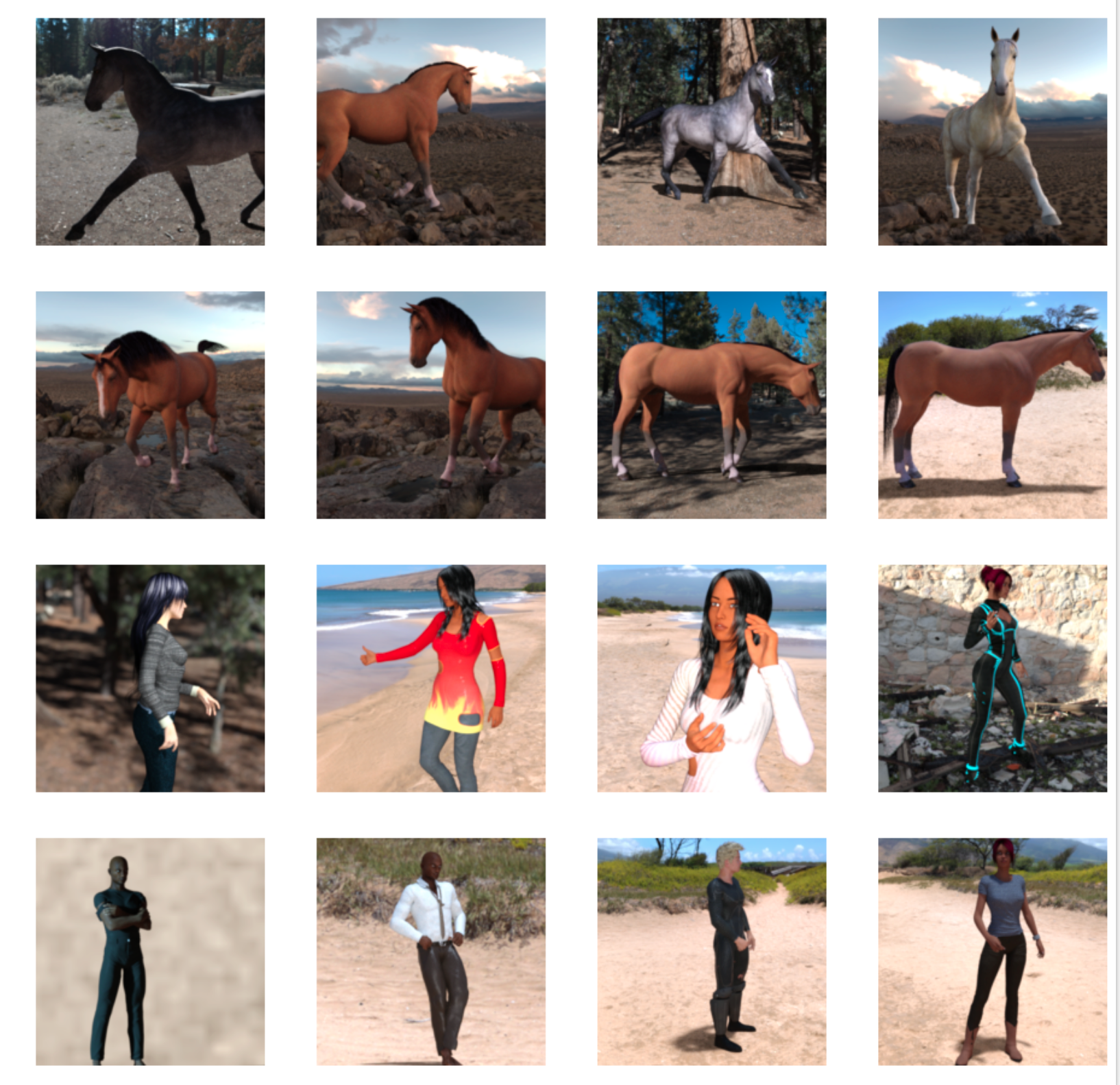
Now, a batch of 8 horses and 8 people are shown. You can rerun the cells to view the new batch each time:
# Set up matplotlib fig, and size it to fit 4x4 pics
fig = plt.gcf()
fig.set_size_inches(ncols * 4, nrows * 4)

pic_index += 8
next_horse_pix = [os.path.join(train_horse_dir, fname)
                for fname in train_horse_names[pic_index-8:pic_index]]
next_human_pix = [os.path.join(train_human_dir, fname)
                for fname in train_human_names[pic_index-8:pic_index]]

for i, img_path in enumerate(next_horse_pix+next_human_pix):
  # Set up subplot; subplot indices start at 1
  sp = plt.subplot(nrows, ncols, i + 1)
  sp.axis('Off') # Don't show axes (or gridlines)

  img = mpimg.imread(img_path)
  plt.imshow(img)

plt.show()
1.1 build a small model from scratch
But before we continue, let's start defining the model:
Step 1 is to import tensorflow.
try:
  # %tensorflow_version only exists in Colab.
  %tensorflow_version 2.x
except Exception:
  pass
import tensorflow as tf
print(tf.__version__)
2.6.0
Then we add the convolution layer as in the previous example and flatten the final result to feed the densely connected layers.
Finally, we add densely connected layers.
Please note that because we are facing a binary classification problem, that is, binary classification problem, we will sigmoid activation End our network, so the output of our network will be a single scalar between 0 and 1, and the coding probability of the current image is class 1 (opposite to class 0).
model = tf.keras.models.Sequential([
    tf.keras.layers.Conv2D(16, (3,3), activation='relu',
                           input_shape=(300, 300, 3)),
    tf.keras.layers.MaxPooling2D(2, 2),
    tf.keras.layers.Conv2D(32, (3,3), activation='relu'),
    tf.keras.layers.MaxPooling2D(2,2),
    tf.keras.layers.Conv2D(64, (3,3), activation='relu'),
    tf.keras.layers.MaxPooling2D(2,2),
    tf.keras.layers.Flatten(),
    tf.keras.layers.Dense(512, activation='relu'),
    tf.keras.layers.Dense(1, activation='sigmoid')
])
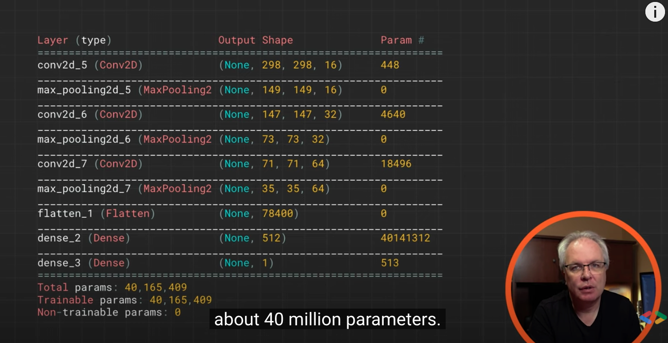
The model.summary() method calls to print a summary of the neural network
model.summary()
Model: "sequential"
_________________________________________________________________
Layer (type)                 Output Shape              Param #
=================================================================
conv2d (Conv2D)              (None, 298, 298, 16)      448
_________________________________________________________________
max_pooling2d (MaxPooling2D) (None, 149, 149, 16)      0
_________________________________________________________________
conv2d_1 (Conv2D)            (None, 147, 147, 32)      4640
_________________________________________________________________
max_pooling2d_1 (MaxPooling2 (None, 73, 73, 32)        0
_________________________________________________________________
conv2d_2 (Conv2D)            (None, 71, 71, 64)        18496
_________________________________________________________________
max_pooling2d_2 (MaxPooling2 (None, 35, 35, 64)        0
_________________________________________________________________
flatten (Flatten)            (None, 78400)             0
_________________________________________________________________
dense (Dense)                (None, 512)               40141312
_________________________________________________________________
dense_1 (Dense)              (None, 1)                 513
=================================================================
Total params: 40,165,409
Trainable params: 40,165,409
Non-trainable params: 0
_________________________________________________________________
The output shape column shows how the size of your feature map evolves in each successive layer. Due to filling, the convolution layer reduces the size of the characteristic graph a little, and the size of each pool layer is halved.
Next, we will configure the specification of model training. We'll use binary_crossentropy loss trains our model because it is a binary classification problem, and our final activation is a sigmoid. (for a review of loss indicators, see Machine learning rmsprop crash course ) we will use an optimizer with a learning rate of 0.001. During the training, we will monitor the classification accuracy.
Note: in this case, use RMSprop optimization algorithm than Random gradient descent (SGD) It is preferable because RMSprop automatically adjusts the learning rate for us. (other optimizers, such as Adam and Adagrad , it will also automatically adjust the learning rate during training, and it can work normally here.)
from tensorflow.keras.optimizers import RMSprop

model.compile(loss='binary_crossentropy',
              optimizer=RMSprop(lr=0.001),
              metrics=['accuracy'])
/usr/local/lib/python3.7/dist-packages/keras/optimizer_v2/optimizer_v2.py:356: UserWarning: The `lr` argument is deprecated, use `learning_rate` instead.
  "The `lr` argument is deprecated, use `learning_rate` instead.")
1.2 data preprocessing
Let's set up a data generator that will read the pictures in our source folder, convert them into float32 tensors, and provide them (with their labels) to our network. We will have a generator for training images and a generator for verifying images. Our generator will generate batch images with a size of 300x300 and their labels (binary).
You may already know that the data entering the neural network should usually be standardized in some way to make it easier for the network to process. (it is not common to input the original pixels into convnet.) in our example, we will preprocess our image by normalizing the pixel values in the range of [0,1] (initially all values are in the range of [0,255]).
In Keras, this can be done through the class of keras.preprocessing.image.ImageDataGenerator using the rescale parameter. This type of ImageDataGenerator allows you to use. flow(data, labels) or instantiate a generator. Flow for enhancing image batches (and their labels)_ from_ directory(directory). These generators can then be used in the Keras model method with accepted data generation as input: fit_generator,evaluate_generator, and predict_generator.
from tensorflow.keras.preprocessing.image import ImageDataGenerator

# All images will be rescaled by 1./255
train_datagen = ImageDataGenerator(rescale=1/255)

# Flow training images in batches of 128 using train_datagen generator
train_generator = train_datagen.flow_from_directory(
        '/tmp/horse-or-human/',  # This is the source directory for training images
        target_size=(300, 300),  # All images will be resized to 150x150
        batch_size=128,
        # Since we use binary_crossentropy loss, we need binary labels
        class_mode='binary')

validation_datagen = ImageDataGenerator(rescale=1/255)

# Flow training images in batches of 128 using train_datagen generator
validation_generator = validation_datagen.flow_from_directory(
        '/tmp/validation-horse-or-human/',  # This is the source directory for training images
        target_size=(300, 300),  # All images will be resized to 150x150
        batch_size=32,
        # Since we use binary_crossentropy loss, we need binary labels
        class_mode='binary')
Found 1027 images belonging to 2 classes.
Found 256 images belonging to 2 classes.
1.3 training
Let's train for 15 periods - this may take a few minutes to run.
Note the value for each period.
Loss and accuracy are good indicators of training progress. It guesses the classification of training data, then measures it according to the known labels and calculates the results. Accuracy is part of the right guess.
history = model.fit(
      train_generator,
      validation_data = validation_generator,
      epochs=15,
      steps_per_epoch=8,
      validation_steps=8,
      verbose=1)
Epoch 1/15
8/8 [==============================] - 41s 1s/step - loss: 5.8897 - accuracy: 0.4705 - val_loss: 0.5922 - val_accuracy: 0.7539
Epoch 2/15
8/8 [==============================] - 8s 1s/step - loss: 0.6112 - accuracy: 0.6885 - val_loss: 1.1099 - val_accuracy: 0.6367
Epoch 3/15
8/8 [==============================] - 8s 1s/step - loss: 0.2795 - accuracy: 0.8587 - val_loss: 3.0112 - val_accuracy: 0.6367
Epoch 4/15
8/8 [==============================] - 8s 1s/step - loss: 0.2430 - accuracy: 0.9021 - val_loss: 1.4884 - val_accuracy: 0.7734
Epoch 5/15
8/8 [==============================] - 8s 1s/step - loss: 0.0752 - accuracy: 0.9689 - val_loss: 4.5065 - val_accuracy: 0.6250
Epoch 6/15
8/8 [==============================] - 8s 1s/step - loss: 0.5074 - accuracy: 0.8576 - val_loss: 4.8991 - val_accuracy: 0.6484
Epoch 7/15
8/8 [==============================] - 10s 1s/step - loss: 0.1014 - accuracy: 0.9677 - val_loss: 1.9106 - val_accuracy: 0.7773
Epoch 8/15
8/8 [==============================] - 9s 1s/step - loss: 0.0136 - accuracy: 0.9980 - val_loss: 2.7661 - val_accuracy: 0.7578
Epoch 9/15
8/8 [==============================] - 9s 1s/step - loss: 0.3347 - accuracy: 0.8701 - val_loss: 1.4895 - val_accuracy: 0.7266
Epoch 10/15
8/8 [==============================] - 8s 1s/step - loss: 0.0438 - accuracy: 0.9878 - val_loss: 1.2067 - val_accuracy: 0.8438
Epoch 11/15
8/8 [==============================] - 8s 1s/step - loss: 0.0137 - accuracy: 0.9967 - val_loss: 2.5188 - val_accuracy: 0.8047
Epoch 12/15
8/8 [==============================] - 8s 1s/step - loss: 0.0026 - accuracy: 1.0000 - val_loss: 2.6172 - val_accuracy: 0.8047
Epoch 13/15
8/8 [==============================] - 8s 1s/step - loss: 0.0023 - accuracy: 1.0000 - val_loss: 2.7464 - val_accuracy: 0.8125
Epoch 14/15
8/8 [==============================] - 8s 1s/step - loss: 0.0159 - accuracy: 0.9933 - val_loss: 29.6021 - val_accuracy: 0.5000
Epoch 15/15
8/8 [==============================] - 9s 1s/step - loss: 3.6140 - accuracy: 0.8242 - val_loss: 1.9420 - val_accuracy: 0.7695
1.4 operation model
Now let's look at actually running the forecast using the model. This code will allow you to select one or more files from the file system, upload them, and run them in the model, indicating whether the object is a horse or a man.
You can download the image from the Internet to your file system for trial!
Please note that you may see that the network has made many mistakes, although the training accuracy is higher than 99%.
This is due to over fitting, which means that the neural network is trained with very limited data - there are only about 500 images in each category. Therefore, it is very good at identifying images similar to those in the training set, but it may fail a lot when identifying images not in the training set.
This is a data point, which proves that the more data you train, the better your final network will be!
Although the data is limited, there are still many technologies that can be used to make your training better, including a technology called image enhancement. This is beyond the scope of this laboratory!
import numpy as np
from google.colab import files
from keras.preprocessing import image

uploaded = files.upload()

for fn in uploaded.keys():

  # predicting images
  path = '/content/' + fn
  img = image.load_img(path, target_size=(300, 300))
  x = image.img_to_array(img)
  x = x / 255
  x = np.expand_dims(x, axis=0)
  images = np.vstack([x])
  classes = model.predict(images, batch_size=10)
  print(classes[0])
  if classes[0]>0.5:
    print(fn + " is a human")
  else:
    print(fn + " is a horse")
You can select multiple pictures at a time

9 files
horse1.jpeg(image/jpeg) - 9533 bytes, last modified: 9/9/2021 - 100% done
horse2.jpeg(image/jpeg) - 6028 bytes, last modified: 9/9/2021 - 100% done
horse3.jpeg(image/jpeg) - 5545 bytes, last modified: 9/9/2021 - 100% done
horse4.jpeg(image/jpeg) - 7278 bytes, last modified: 9/9/2021 - 100% done
lady1.jpeg(image/jpeg) - 5549 bytes, last modified: 9/9/2021 - 100% done
lady2.jpeg(image/jpeg) - 5713 bytes, last modified: 9/9/2021 - 100% done
lady3.jpeg(image/jpeg) - 8627 bytes, last modified: 9/9/2021 - 100% done
lady4.jpeg(image/jpeg) - 6872 bytes, last modified: 9/9/2021 - 100% done
lady5.jpeg(image/jpeg) - 5807 bytes, last modified: 9/9/2021 - 100% done
Saving horse1.jpeg to horse1 (1).jpeg
Saving horse2.jpeg to horse2.jpeg
Saving horse3.jpeg to horse3.jpeg
Saving horse4.jpeg to horse4.jpeg
Saving lady1.jpeg to lady1.jpeg
Saving lady2.jpeg to lady2.jpeg
Saving lady3.jpeg to lady3.jpeg
Saving lady4.jpeg to lady4.jpeg
Saving lady5.jpeg to lady5.jpeg
[0.34198874]
horse1.jpeg is a horse
[2.307064e-07]
horse2.jpeg is a horse
[0.15786135]
horse3.jpeg is a horse
[0.99264127]
horse4.jpeg is a human
[0.0008325]
lady1.jpeg is a horse
[0.04066621]
lady2.jpeg is a horse
[1.406738e-09]
lady3.jpeg is a horse
[0.9999918]
lady4.jpeg is a human
[0.4901081]
lady5.jpeg is a horse
1.5 visual intermediate representation
In order to understand what features our convnet has learned, an interesting thing is how visual input is converted through convnet.
Let's randomly select an image from the training set, and then generate a graph. Each row is the output of a layer, and each image in the row is a specific filter in the output feature graph. Rerun this cell to generate an intermediate representation of the various training images.
import numpy as np
import random
from tensorflow.keras.preprocessing.image import img_to_array, load_img

# Let's define a new Model that will take an image as input, and will output
# intermediate representations for all layers in the previous model after
# the first.
successive_outputs = [layer.output for layer in model.layers[1:]]
#visualization_model = Model(img_input, successive_outputs)
visualization_model = tf.keras.models.Model(inputs = model.input, outputs = successive_outputs)
# Let's prepare a random input image from the training set.
horse_img_files = [os.path.join(train_horse_dir, f) for f in train_horse_names]
human_img_files = [os.path.join(train_human_dir, f) for f in train_human_names]
img_path = random.choice(horse_img_files + human_img_files)

img = load_img(img_path, target_size=(300, 300))  # this is a PIL image
x = img_to_array(img)  # Numpy array with shape (150, 150, 3)
x = x.reshape((1,) + x.shape)  # Numpy array with shape (1, 150, 150, 3)

# Rescale by 1/255
x /= 255

# Let's run our image through our network, thus obtaining all
# intermediate representations for this image.
successive_feature_maps = visualization_model.predict(x)

# These are the names of the layers, so can have them as part of our plot
layer_names = [layer.name for layer in model.layers]

# Now let's display our representations
for layer_name, feature_map in zip(layer_names, successive_feature_maps):
  if len(feature_map.shape) == 4:
    # Just do this for the conv / maxpool layers, not the fully-connected layers
    n_features = feature_map.shape[-1]  # number of features in feature map
    # The feature map has shape (1, size, size, n_features)
    size = feature_map.shape[1]
    # We will tile our images in this matrix
    display_grid = np.zeros((size, size * n_features))
    for i in range(n_features):
      # Postprocess the feature to make it visually palatable
      x = feature_map[0, :, :, i]
      x -= x.mean()
      # if x>0:
      #   x /= x.std()
      x *= 64
      x += 128
      x = np.clip(x, 0, 255).astype('uint8')
      # We'll tile each filter into this big horizontal grid
      display_grid[:, i * size : (i + 1) * size] = x
    # Display the grid
    scale = 20. / n_features
    plt.figure(figsize=(scale * n_features, scale))
    plt.title(layer_name)
    plt.grid(False)
    plt.imshow(display_grid, aspect='auto', cmap='viridis')
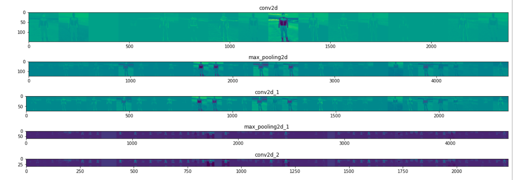
As you can see, we move from the original pixels of the image to an increasingly abstract and compact representation. Downstream representations begin to highlight the content concerned by the network, and they show that fewer and fewer features are "activated"; Most are set to zero. This is called sparsity. Representation sparsity is a key feature of deep learning.
These representations carry less and less information about the original pixels of the image, but more and more fine information about the image category. You can think of convnet (or general deep network) as an information distillation pipeline.
1.6 cleaning
Before running the next exercise, run the following cells to terminate the kernel and free up memory resources:
import os, signal
os.kill(os.getpid(), signal.SIGKILL)
reference resources
https://www.youtube.com/watch?v=0kYIZE8Gl90