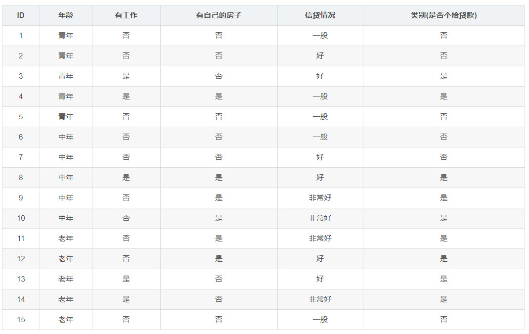
Given a table, how to reasonably analyze these 15 groups of data and mine their relationship with the results? Given a situation, how to predict the result (loan or not)?
All codes are as follows:
# -*- coding: UTF-8 -*-
from matplotlib.font_manager import FontProperties
import matplotlib.pyplot as plt
from math import log
import operator


def calcShannonEnt(dataSet):                        #Calculate Shannon entropy
	numEntires = len(dataSet)						#Returns the number of rows in the dataset
	labelCounts = {}								#Save a dictionary of the number of occurrences of each label
	for featVec in dataSet:							#Make statistics for each group of eigenvectors
		currentLabel = featVec[-1]					#Extract label information
		if currentLabel not in labelCounts.keys():	#If the label is not put into the dictionary of statistical times, add it
			labelCounts[currentLabel] = 0
		labelCounts[currentLabel] += 1				#Label count
	shannonEnt = 0.0								#Empirical entropy (Shannon entropy)
	for key in labelCounts:							#Calculate Shannon entropy
		prob = float(labelCounts[key]) / numEntires	#The probability of selecting the label
		shannonEnt -= prob * log(prob, 2)			#Calculate by formula
	return shannonEnt								#Return empirical entropy (Shannon entropy)


def createDataSet():                                #Create dataset
	dataSet = [[0, 0, 0, 0, 'no'],						#data set
			[0, 0, 0, 1, 'no'],                       #list is a two-dimensional array
			[0, 1, 0, 1, 'yes'],
			[0, 1, 1, 0, 'yes'],
			[0, 0, 0, 0, 'no'],
			[1, 0, 0, 0, 'no'],
			[1, 0, 0, 1, 'no'],
			[1, 1, 1, 1, 'yes'],
			[1, 0, 1, 2, 'yes'],
			[1, 0, 1, 2, 'yes'],
			[2, 0, 1, 2, 'yes'],
			[2, 0, 1, 1, 'yes'],
			[2, 1, 0, 1, 'yes'],
			[2, 1, 0, 2, 'yes'],
			[2, 0, 0, 0, 'no']]
	labels = ['Age', 'Have a job', 'Have your own house', 'Credit situation']		#Feature tags, labels is a list type with a list stored
	return dataSet, labels 							#Return dataset and classification properties


def splitDataSet(dataSet, axis, value):		#Segment data sets according to characteristics
	retDataSet = []										#Create a list of returned datasets
	for featVec in dataSet: 							#Traversal data set
		if featVec[axis] == value:
			reducedFeatVec = featVec[:axis]				#Remove axis feature
			reducedFeatVec.extend(featVec[axis+1:]) 	#Add eligible to the returned dataset
			retDataSet.append(reducedFeatVec)
	return retDataSet		  							#Returns the divided dataset


def chooseBestFeatureToSplit(dataSet):                  #Find the feature with the largest information gain of the root node and remove it
	numFeatures = len(dataSet[0]) - 1					#Number of features, len(dataSet[0]) returns the number of columns of this two-dimensional array, and numFeatures is equal to 4
	baseEntropy = calcShannonEnt(dataSet) 				#Shannon entropy of calculated data set, 0.971
	bestInfoGain = 0.0  								#information gain
	bestFeature = -1									#Index value of optimal feature
	for i in range(numFeatures): 						#Traverse all features
		#Get the i th all features of dataSet
		featList = [example[i] for example in dataSet]  #Take out each column of the array and assign it to featList
		uniqueVals = set(featList)     					#Create set set {}, and the element cannot be repeated, that is {0,1,2}
		newEntropy = 0.0  								#Empirical conditional entropy
		for value in uniqueVals: 						#Calculate information gain
			subDataSet = splitDataSet(dataSet, i, value) 		#Subset after sub dataset partition
			prob = len(subDataSet) / float(len(dataSet))   		#Calculate the probability of subset
			newEntropy += prob * calcShannonEnt(subDataSet) 	#The empirical conditional entropy is calculated according to the formula
		infoGain = baseEntropy - newEntropy 					#information gain
		# print("The first%d The gain of each feature is%.3f" % (i, infoGain))			#Print information gain for each feature
		if (infoGain > bestInfoGain): 							#Calculate information gain
			bestInfoGain = infoGain 							#Update the information gain and find the maximum information gain
			bestFeature = i 									#Record the index value of the feature with the largest information gain
	return bestFeature 											#Returns the index value of the feature with the largest information gain


def majorityCnt(classList):                            #vote by ballot
	classCount = {}
	for vote in classList:										#Count the number of occurrences of each element in the classList
		if vote not in classCount.keys():classCount[vote] = 0
		classCount[vote] += 1
	sortedClassCount = sorted(classCount.items(), key = operator.itemgetter(1), reverse = True)		#Sort in descending order according to the values of the dictionary
	return sortedClassCount[0][0]								#Returns the most frequent element in the classList


def createTree(dataSet, labels, featLabels):                  #Core program, create tree
	classList = [example[-1] for example in dataSet]			#Take the classification label (lending or not: yes or no)
	if classList.count(classList[0]) == len(classList):			#If the categories are exactly the same, stop dividing, which means that if they are all yes or no, there is nothing to decide. That's the end
		return classList[0]
	if len(dataSet[0]) == 1 or len(labels) == 0:				#When all features are traversed, the class label with the most occurrences is returned. If all features are not enough to determine the result, it ends
		return majorityCnt(classList)
	bestFeat = chooseBestFeatureToSplit(dataSet)				#Select the optimal feature
	bestFeatLabel = labels[bestFeat]							#Optimal feature label
	featLabels.append(bestFeatLabel)
	myTree = {bestFeatLabel:{}}									#Label spanning tree based on optimal features
	del(labels[bestFeat])										#Delete used feature labels
	featValues = [example[bestFeat] for example in dataSet]		#The attribute values of all optimal features in the training set are obtained
	uniqueVals = set(featValues)								#Remove duplicate attribute values
	for value in uniqueVals:									#Traverse the features and create a decision tree.
		subLabels = labels[:]
		myTree[bestFeatLabel][value] = createTree(splitDataSet(dataSet, bestFeat, value), subLabels, featLabels)

	return myTree

def classify(inputTree, featLabels, testVec):
	firstStr = next(iter(inputTree))														#Get decision tree node
	secondDict = inputTree[firstStr]														#Next dictionary
	featIndex = featLabels.index(firstStr)
	for key in secondDict.keys():
		if testVec[featIndex] == key:
			if type(secondDict[key]).__name__ == 'dict':
				classLabel = classify(secondDict[key], featLabels, testVec)
			else: classLabel = secondDict[key]
	return classLabel

if __name__ == '__main__':
	dataSet, labels = createDataSet()
	featLabels = []
	myTree = createTree(dataSet, labels, featLabels)
	testVec = [0,1]										#test data
	result = classify(myTree, featLabels, testVec)
	if result == 'yes':
		print('lending')
	if result == 'no':
		print('No lending')
Whether it is "age", "work", "house" or "credit", it is more or less related to the result of "lending". So, which factor is more important? If the bank's judgment is based on the internal tree structure of the bank, just like the kind of psychological test that I played when I was a child. When I met a question, I turned to how many pages and finally gave an answer, what kind of tree is it?
I don't know the specific form of the tree, but I know that if we build such a tree, we need to put the one that has the greatest impact on the results in the front, and the greater the effect, the more we need to be in the front, which is reasonable. So how to define the influence of factors?
The judgment method is information gain:

g(D,A) represents the influence of A on D, and H (d) and H (D|A) are entropy. Entropy, as mentioned in high school chemistry, indicates the degree of chaos. There is no doubt that the entropy of gas is greater than that of liquid. In information theory, it refers to the degree of confusion of information. The more chaotic it is, the more irrelevant it is. On the contrary, if there is no confusion, it means that the relationship between the two is closer. If the fitting curve is A straight line, the correlation coefficient of high school mathematics is 1, and then it is A straight line in the rectangular coordinate diagram, it means that the linear constraint between the two has reached the degree that you and I decide each other and have nothing to do with others. If it really reaches this level, then H (D|A) is very small, so g(D,A) is very large. Therefore, to establish A planning tree, these influencing factors need to be sorted according to information gain. The greater the information gain, the higher the information gain.
First, execute the main function and get 15 groups of data and corresponding factor names from dataSet labels. Declare a featLabels array, which is intended to hold the names of influencing factors in order. Then enter the sub function createTree()
def createTree(dataSet, labels, featLabels):                  #Core program, create tree
	classList = [example[-1] for example in dataSet]			#Take the classification label (lending or not: yes or no)
	if classList.count(classList[0]) == len(classList):			#If the categories are exactly the same, stop dividing, which means that if they are all yes or no, there is nothing to decide. That's the end
		return classList[0]
	if len(dataSet[0]) == 1 or len(labels) == 0:				#When all features are traversed, the class label with the most occurrences is returned. If all features are not enough to determine the result, it ends
		return majorityCnt(classList)
	bestFeat = chooseBestFeatureToSplit(dataSet)				#Select the optimal feature
	bestFeatLabel = labels[bestFeat]							#Optimal feature label
	featLabels.append(bestFeatLabel)
	myTree = {bestFeatLabel:{}}									#Label spanning tree based on optimal features
	del(labels[bestFeat])										#Delete used feature labels
	featValues = [example[bestFeat] for example in dataSet]		#The attribute values of all optimal features in the training set are obtained
	uniqueVals = set(featValues)								#Remove duplicate attribute values
	for value in uniqueVals:									#Traverse the features and create a decision tree.
		subLabels = labels[:]
		myTree[bestFeatLabel][value] = createTree(splitDataSet(dataSet, bestFeat, value), subLabels, featLabels)
	return myTree
This function is not only the core program of building a planning tree, but also a recursive program. After all, it is to build a tree. classList gets the last element of 15 groups of data, that is, the judgment result. Here are two if statements. These two if statements are the closing statements of the recursive function. The first if means that if all the results are the same, there are no influencing factors at all. Naturally, this situation needs to be eliminated. The second if means that if the loop traverses all factors and still cannot judge the situation (it may need to be judged in other situations, and these factors alone are not enough), then the most results among all results will be returned. After all, these training sets alone cannot judge, but can only give you a more likely result.
Then enter the chooseBestFeatureToSplit() function
def chooseBestFeatureToSplit(dataSet):                  #Find the feature with the largest information gain of the root node and remove it
	numFeatures = len(dataSet[0]) - 1					#Number of features, len(dataSet[0]) returns the number of columns of this two-dimensional array, and numFeatures is equal to 4
	baseEntropy = calcShannonEnt(dataSet) 				#Shannon entropy of calculated data set, 0.971
	bestInfoGain = 0.0  								#information gain
	bestFeature = -1									#Index value of optimal feature
	for i in range(numFeatures): 						#Traverse all features
		#Get the i th all features of dataSet
		featList = [example[i] for example in dataSet]  #Take out each column of the array and assign it to featList
		uniqueVals = set(featList)     					#Create set set {}, and the element cannot be repeated, that is {0,1,2}
		newEntropy = 0.0  								#Empirical conditional entropy
		for value in uniqueVals: 						#Calculate information gain
			subDataSet = splitDataSet(dataSet, i, value) 		#Subset after sub dataset partition
			prob = len(subDataSet) / float(len(dataSet))   		#Calculate the probability of subset
			newEntropy += prob * calcShannonEnt(subDataSet) 	#The empirical conditional entropy is calculated according to the formula
		infoGain = baseEntropy - newEntropy 					#information gain
		# print("The first%d The gain of each feature is%.3f" % (i, infoGain))			#Print information gain for each feature
		if (infoGain > bestInfoGain): 							#Calculate information gain
			bestInfoGain = infoGain 							#Update the information gain and find the maximum information gain
			bestFeature = i 									#Record the index value of the feature with the largest information gain
	return bestFeature 											#Returns the index value of the feature with the largest information gain
numFeatures gets the number of all factors that affect the results. Then we call Shannon function to calculate Shannon entropy, that is, H (D). This function needs to store keywords and times in the form of a dictionary. For these 15 groups of data, there are 15 results, 9 "yes" and 6 "no", so the calculation result is

Enter the for loop. featList obtains the i-th column of the dataSet and forms an array by itself. uniqyeVals is obtained after non repetition. After entering the nested loop, the splitDataSet() function splits the dataSet and calculates the newentry, that is, H (D|A). Then subtract to get the information gain. The subsequent if statement is used to save the serial number of the factor where the largest information capital increase is located. At this point, the serial number is returned.
After a lot of hard work, we finally got the biggest factor affecting the result. Return to the createTree () function. The labels function deletes the corresponding element, and the fearList receives this element. uniqueVals gets all the elements of the optimal feature (no repetition). Then use the for loop to recurse on each node and continue to generate the tree. Continue to find the second largest optimal feature, build a tree, continue to find Until those two if conditions are met.
In this way, such a tree has been built. What is this tree like? There are only two floors, not the four floors generally thought. Because in fact, two factors "house" and "work" can already determine the result. House is the best feature, followed by work. If more than one of the two is satisfied, it is "yes", otherwise, "no". After that, the newly given situation is verified by the classify() function. testVec = [0,1], of course "yes" because he has a job.
Does anyone have such an idea? Set up dictionary sorting in the chooseBestFeatureToSplit() function, directly find the information gain of each factor in this function and arrange the order directly. I thought so at first, but later I thought it was wrong. For recursive statements in the createTree() function
myTree[bestFeatLabel][value] = createTree(splitDataSet(dataSet, bestFeat, value), subLabels, featLabels)
splitDataSet() function to separate the optimal features. The subsequent information gain is independent of the optimal feature. If the information gain is calculated directly in the chooseBestFeatureToSplit() function, the information gain of other factors will be related to the optimal feature. The internal connection has not been cut off. This is wrong.