1. Likelihood function of GMM
about
K
=
3
,
μ
=
[
(
1
,
1
)
(
3
,
3
)
(
5
,
5
)
]
,
c
o
v
=
[
(
1
−
0.8
−
0.8
1
)
(
1
0.8
0.8
1
)
(
1
−
0.8
−
0.8
1
)
]
K=3\ ,\ \mu=\begin{bmatrix} (1,1)\\(3,3)\\(5,5)\end{bmatrix}, cov=\begin{bmatrix}\begin{pmatrix}1&-0.8\\-0.8&1\end{pmatrix}\\\begin{pmatrix}1&0.8\\0.8&1\end{pmatrix}\\\begin{pmatrix}1&-0.8\\-0.8&1\end{pmatrix}\end{bmatrix}
K=3 , μ=⎣⎡(1,1)(3,3)(5,5)⎦⎤,cov=⎣⎢⎢⎢⎢⎢⎢⎡(1−0.8−0.81)(10.80.81)(1−0.8−0.81)⎦⎥⎥⎥⎥⎥⎥⎤
The mixing ratio is
w
∼
D
i
r
i
c
h
l
e
t
(
α
)
,
α
=
(
8
,
4
,
8
)
w\sim Dirichlet(\alpha)\ ,\ \alpha=(8,4,8)
w∼Dirichlet( α) , α= (8,4,8), PM can be used in PyMC3 Mix or PM Densitydist to construct likelihood function and extract samples.
First, construct and analyze the data as a reference.
%matplotlib inline
import arviz as az
import matplotlib.pyplot as plt
import numpy as np
import pandas as pd
import pymc3 as pm
import theano.tensor as tt
import seaborn as sns
from sklearn import mixture
import dill, theano
from scipy.stats import multivariate_normal as mvn
x,y = np.mgrid[-3:9:0.1, -3:9:0.1]
pos = np.dstack((x,y))
com1 = mvn(means[0],cov[0]).pdf(pos)
com2 = mvn(means[1],cov[1]).pdf(pos)
com3 = mvn(means[2],cov[2]).pdf(pos)
liklihood_function = w[0]*com1 + w[1]*com2 + w[2]*com3
fig = plt.figure(1)
ax = fig.add_subplot(111)
ax.contourf(x,y,liklihood_function,levels=100,cmap='jet')
ax.scatter(x=means[:,0], y=means[:,1], color='white', edgecolor='black')
plt.title('GMM Analytical, K=3')
plt.show()
Operation results:
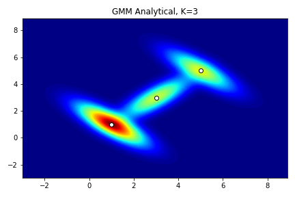
The goal of constructing likelihood function is not to estimate, but to stably produce more accurate samples, so we should provide as many and accurate parameters as possible for the model.
1.1 use PM Mixture
In order to reduce the burden of PyMC3 reasoning, the parameters are assigned outside the model as much as possible.
K=3
means = np.array([1,1,3,3,5,5]).reshape((3,2))
cov = np.array([1, -0.8, -0.8, 1, 1, 0.8, 0.8, 1, 1, -0.8, -0.8, 1]).reshape((3,2,2))
alpha = np.array([8, 4, 8])
w = np.random.dirichlet(alpha)

with pm.Model() as model:
	comp1 = pm.MvNormal.dist(mu=means[0], cov=cov[0], shape=2)
	comp2 = pm.MvNormal.dist(mu=means[1], cov=cov[1], shape=2)
	comp3 = pm.MvNormal.dist(mu=means[2], cov=cov[2], shape=2)
	liklihood = pm.Mixture('liklihood', w=w, comp_dists=[comp1, comp2, comp3], shape=2)
Use Slice sampling and convert the track to DataFrame, using Seaborn Join plot to view the sampling results:
with model:
	trace = pm.sample(2000, step=pm.Slice(), tune=2000, pickle_backend='dill')
	dftrace = pm.trace_to_dataframe(trace)
sns.jointplot(data=dftrace, x='liklihood__0', y='liklihood__1', kind='hex')
Operation results:
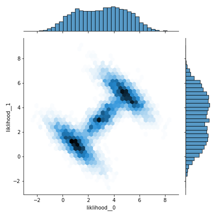
The results are basically consistent with the analytical data.
1.2 use PM DensityDist
After constructing the analytic function with theano, specify the log likelihood function, and finally pass PM Densitydist is specified as the likelihood function.
#Constructing analytic likelihood function
cov_inverse = np.linalg.inv(cov)
z = tt.matrix('z')
z.tag.test_value=pm.floatX([0,0])
def gmm2dliklihood(z):
    z = z.T
    comp1 = 1/np.sqrt(2*np.pi*np.linalg.det(cov)[0])*np.exp(-1/2*(
         (z[0]-means[0,0])**2*cov_inverse[0,0,0]
        +(z[0]-means[0,0])*(z[1]-means[0,1])*cov_inverse[0,0,1]
        +(z[1]-means[0,1])*(z[0]-means[0,0])*cov_inverse[0,1,0]
        +(z[1]-means[0,1])**2*cov_inverse[0,1,1]))
    comp2 = 1/np.sqrt(2*np.pi*np.linalg.det(cov)[1])*np.exp(-1/2*(
         (z[0]-means[1,0])**2*cov_inverse[1,0,0]
        +(z[0]-means[1,0])*(z[1]-means[1,1])*cov_inverse[1,0,1]
        +(z[1]-means[1,1])*(z[0]-means[1,0])*cov_inverse[1,1,0]
        +(z[1]-means[1,1])**2*cov_inverse[1,1,1]))
    comp3 = 1/np.sqrt(2*np.pi*np.linalg.det(cov)[2])*np.exp(-1/2*(
         (z[0]-means[2,0])**2*cov_inverse[2,0,0]
        +(z[0]-means[2,0])*(z[1]-means[2,1])*cov_inverse[2,0,1]
        +(z[1]-means[2,1])*(z[0]-means[2,0])*cov_inverse[2,1,0]
        +(z[1]-means[2,1])**2*cov_inverse[2,1,1]))
    return w[0]*comp1 + w[1]*comp2 + w[2]*comp3
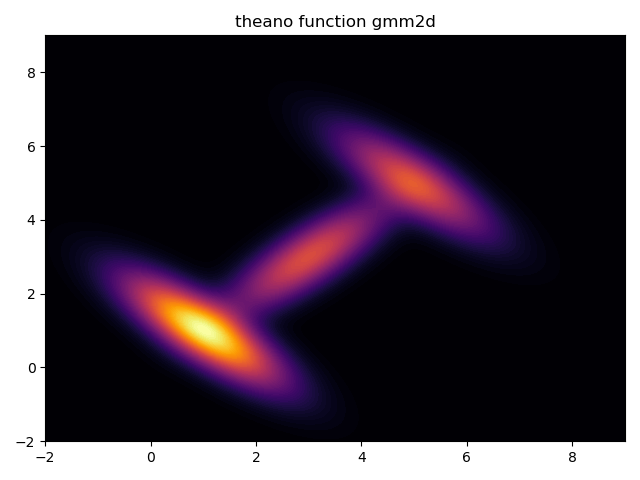
First, determine whether the constructed likelihood function is correct:
gmm2dliklihood_plot = theano.function([z],gmm2dliklihood(z))
grid = pm.floatX(np.mgrid[ -2:9:1000j, -2:9:1000j])
grid2d = grid.reshape(2, -1).T
pdf = gmm2dliklihood_plot(grid2d)
plt.contourf(grid[0], grid[1], pdf.reshape(1000, 1000), cmap='inferno',levels=80)
plt.title('theano function gmm2d')
plt.show()
Operation results:
from pymc3.distributions.dist_math import bound
#Constructing log likelihood function
def gmmlogp(z):
    return np.log(gmm2dliklihood(z))
#Pass both likelihood functions into the model, use Slice sampling and convert them to DataFrame
with pm.Model() as model:
    gmm2dlike = pm.DensityDist("gmm2dlike", logp=gmmlogp, shape=(2,))
    trace = pm.sample(2000, step=pm.Slice(), tune=2000, pickle_backend='dill')
    dftrace = pm.trace_to_dataframe(trace)
#View through jointplot
sns.jointplot(data=dftrace, x='gmm2dlike__0', y='gmm2dlike__1', kind='hex', cmap='Reds')
Operation results:
Multiprocess sampling (4 chains in 4 jobs)
Slice: [gmm2dlike]

 100.00% [16000/16000 00:11<00:00 Sampling 4 chains, 0 divergences]
Sampling 4 chains for 2_000 tune and 2_000 draw iterations (8_000 + 8_000 draws total) took 30 seconds.
The number of effective samples is smaller than 10% for some parameters.
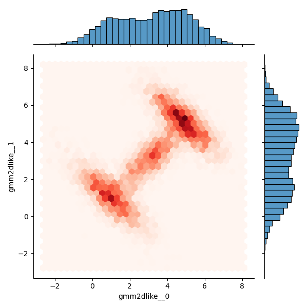
It is basically consistent with the analytical data and the results in 1.1, but it is too slow to generate samples through these two methods, and a faster method should be considered.
2. Use sklearn's GMM as a fast sample generator
Using sklearn's GMM as a fast sample generator will bring many convenience in practice. For example, when we need 100000 or more GMM likelihood function sample points, we do not need to pass pymc3 Sample performs long MCMC sampling, but uses sklearn's GMM fitting according to a small number of MCMC samples, and finally quickly generates a large number of samples, so as to save time.
from sklearn import mixture
skgmm = mixture.GaussianMixture(n_components=K
                                , covariance_type='full'
                                , weights_init=w
                                ,means_init=means
                               )
skgmm.fit(trace['liklihood'])
sksamples, index = skgmm.sample(10000000)
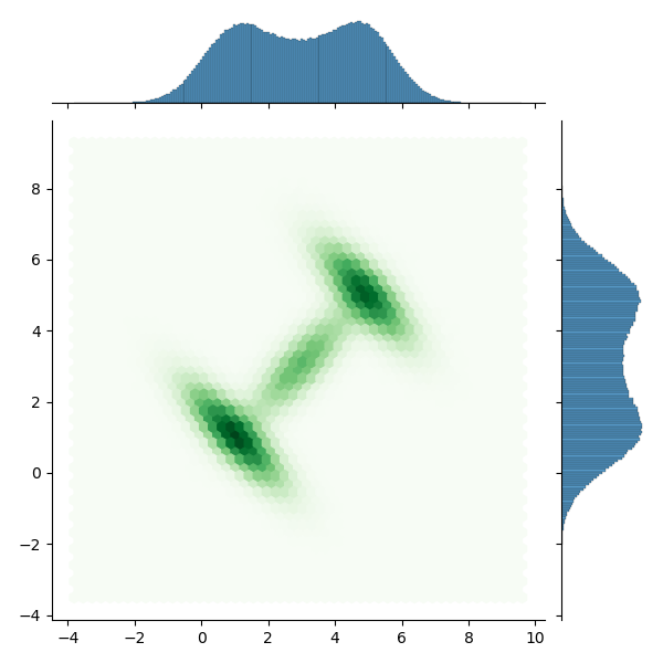
sns.jointplot(x=sksamples[:,0], y=sksamples[:,1], kind='hex', cmap='Greens')
You can check the difference between the two by timing. The same GMM likelihood function still generates 1000000 samples:
with pm.Model() as model:
	comp1 = pm.MvNormal.dist(mu=means[0], cov=cov[0], shape=2)
	comp2 = pm.MvNormal.dist(mu=means[1], cov=cov[1], shape=2)
	comp3 = pm.MvNormal.dist(mu=means[2], cov=cov[2], shape=2)
	liklihood = pm.Mixture('liklihood', w=w, comp_dists=[comp1, comp2, comp3], shape=2)
	trace = pm.sample(1000000, step=pm.Slice(), tune=2000, pickle_backend='dill')
	dftrace = pm.trace_to_dataframe(trace)
Operation results:
Multiprocess sampling (4 chains in 4 jobs)
Slice: [liklihood]
100.00% [4008000/4008000 47:17<00:00 Sampling 4 chains, 0 divergences]
Sampling 4 chains for 2_000 tune and 1_000_000 draw iterations (8_000 + 4_000_000 draws total) took 2856 seconds.
The number of effective samples is smaller than 10% for some parameters.
Or this way:
cov_inverse = np.linalg.inv(cov)
z = tt.matrix('z')
z.tag.test_value=pm.floatX([0,0])
def gmm2dliklihood(z):
    z = z.T
    comp1 = 1/np.sqrt(2*np.pi*np.linalg.det(cov)[0])*np.exp(-1/2*(
         (z[0]-means[0,0])**2*cov_inverse[0,0,0]
        +(z[0]-means[0,0])*(z[1]-means[0,1])*cov_inverse[0,0,1]
        +(z[1]-means[0,1])*(z[0]-means[0,0])*cov_inverse[0,1,0]
        +(z[1]-means[0,1])**2*cov_inverse[0,1,1]))
    comp2 = 1/np.sqrt(2*np.pi*np.linalg.det(cov)[1])*np.exp(-1/2*(
         (z[0]-means[1,0])**2*cov_inverse[1,0,0]
        +(z[0]-means[1,0])*(z[1]-means[1,1])*cov_inverse[1,0,1]
        +(z[1]-means[1,1])*(z[0]-means[1,0])*cov_inverse[1,1,0]
        +(z[1]-means[1,1])**2*cov_inverse[1,1,1]))
    comp3 = 1/np.sqrt(2*np.pi*np.linalg.det(cov)[2])*np.exp(-1/2*(
         (z[0]-means[2,0])**2*cov_inverse[2,0,0]
        +(z[0]-means[2,0])*(z[1]-means[2,1])*cov_inverse[2,0,1]
        +(z[1]-means[2,1])*(z[0]-means[2,0])*cov_inverse[2,1,0]
        +(z[1]-means[2,1])**2*cov_inverse[2,1,1]))
    return w[0]*comp1 + w[1]*comp2 + w[2]*comp3
def gmmlogp(z):
    return np.log(gmm2dliklihood(z))
with pm.Model() as model:
    gmm2dlike = pm.DensityDist("gmm2dlike", logp=gmmlogp, shape=(2,))
    trace = pm.sample(1000000, step=pm.Slice(), tune=2000, pickle_backend='dill')
    dftrace = pm.trace_to_dataframe(trace)
Operation results:
Multiprocess sampling (4 chains in 4 jobs)
Slice: [gmm2dlike]
100.00% [4008000/4008000 24:18<00:00 Sampling 4 chains, 0 divergences]
Sampling 4 chains for 2_000 tune and 1_000_000 draw iterations (8_000 + 4_000_000 draws total) took 1475 seconds.
The number of effective samples is smaller than 10% for some parameters.
It takes a long time, and the method of using a small number of samples + sklearnGMM:
from pymc3.distributions.dist_math import bound
from sklearn import mixture
def gmmlogp(z):
    return np.log(gmm2dliklihood(z))
with pm.Model() as model:
    gmm2dlike = pm.DensityDist("gmm2dlike", logp=gmmlogp, shape=(2,))
    trace = pm.sample(400, step=pm.Slice(), pickle_backend='dill')
    dftrace = pm.trace_to_dataframe(trace)
Only 400 samples in chain.
Multiprocess sampling (4 chains in 4 jobs)
Slice: [gmm2dlike]

100.00% [5600/5600 00:06<00:00 Sampling 4 chains, 0 divergences]
Sampling 4 chains for 1_000 tune and 400 draw iterations (4_000 + 1_600 draws total) took 23 seconds.
The rhat statistic is larger than 1.05 for some parameters. This indicates slight problems during sampling.
The estimated number of effective samples is smaller than 200 for some parameters.
%%time
skgmm = mixture.GaussianMixture(n_components=K
                                , covariance_type='full'
                                , weights_init=w
                                ,means_init=means)

skgmm.fit(trace['gmm2dlike'])
sksamples, index = skgmm.sample(1000000)
sns.jointplot(data=dftrace, x='gmm2dlike__0', y='gmm2dlike__1', kind='hex', cmap='Reds')
Wall time: 173 ms
Operation results:
