This article is a translation learning article for learning. The models and instructions in this article have been redrawn and tested, and can be used.
Original address: https://ww2.mathworks.cn/help/ident/ug/estimating-transfer-function-models-for-a-boost-converter.html
This example shows how to estimate the transfer function from frequency response data. You can collect the frequency response model of a Simulink model through silmulink contract design, and then use the tftest instruction to estimate a transfer function based on the measured data. If you need to know how to estimate the transfer function from the frequency response data obtained in advance, you can skip directly to the estimation transfer function section.

boost converter

Open the simulink model.

mdl = 'iddemo_boost_converter';									
Open_system(mdl);	

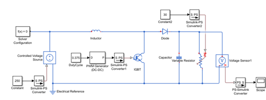
This model is a boost conversion line that converts DC voltage to another DC voltage (usually higher voltage) through switching voltage source control. In this model, IGBT is driven by PWM signal as a switch.
For this example, we are interested in the transfer function Uout from the PWM duty cycle setpoint to the load voltage.

Collect frequency response data

We use the frestimate command to perturb the duty cycle set point through sinusoids of different frequencies, and record the generated load voltage at the same time. In this way, we can find out how the system changes the amplitude and phase of the injected sinusoidal signal, so as to provide us with discrete points of frequency response.
Using freshmate requires two initial steps:
1. Select the input and output points of frequency response;
2. The sinusoidal injection point is defined at the input;
The input and output points of frequency response are created by using the linio command. For this example, the output and voltage measurement module of DutyCycle.

ios = [...
   		 linio([mdl,'/DutyCycle'],1,'input'); ...
    	 linio([mdl,'/PS-Simulink Converter'],1,'output')];

We use frost Sinestream command to define sinusoidal signal injection at the input point. We are interested in the frequency range of 200-20K rad/s and want to disturb the duty cycle by 0.03.

F = logspace(log10(200),log10(20000),10); 
in = frest.Sinestream('Frequency',f,'Amplitude',0.03);

The simulation time using the sinusoidal signal simulation model is determined by getSimulationTime. Since we know the simulation end time used by the model, we can understand how long the sinusoidal flow simulation will take up the simplified operation of the model.

getSimulationTime(in)/0.02

We calculate the discrete points of the frequency response by using the defined input and sinusoidal flow.

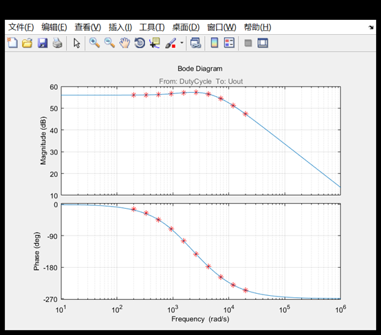
[sysData,simlog] = frestimate(mdl,ios,in); 
bopt               = bodeoptions; 
bopt.Grid          = 'on'; 
bopt.PhaseMatching = 'on'; 
figure, bode(sysData,'*r',bopt)

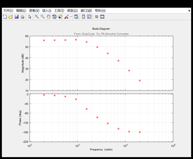
The baud diagram shows that the system gain is 56 dB and there are some resonances near 2500 rad / s. The high-frequency part drops at 20db / ten times the frequency, which matches our expectations for the circuit.
Frest. The simview command allows us to check the freshmate process in a graphical interface showing the injection signal, output measurement and frequency response.

frest.simView(simlog,in,sysData);

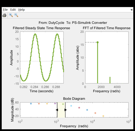
This picture shows the frequency response of the model corresponding to the injected signal and the FFT of the model response. Note that the resulting signal injected with sinusoidal waveform has dominant frequency and finite harmonic, indicating that the model is a linear model, and the frequency response data are successfully collected.

Estimate a transfer function

Through the previous steps, we collected the frequency response data. These data describe a system with discrete frequency points. We can now use the transfer function to match the data.
We can generate frequency response data through Simulink contract design. If Simulink contract design is not installed, we can load the saved frequency response data through the following command.

load iddemo_boostconverter_data

By examining the frequency response data, we evaluate that the system may be described as a second-order system.

sysA = tfest(sysData,2) 
figure, bode(sysData,'r*',sysA,bopt)

sysA =     

From input "DutyCycle" to output "PS-Simulink Converter":   
-4.456e06 s + 6.175e09   
----------------------  
s^2 + 6995 s + 9.834e06   

Continuous-time identified transfer function.
Parameterization:    
Number of poles: 2   
Number of zeros: 1    
Number of free coefficients: 4    
Use "tfdata", "getpvec", "getcov" for parameters and their uncertainties.

Status:                                                     
Estimated using TFEST on frequency response data "sysData".
Fit to estimation data: 98.04%                              
FPE: 281.4, MSE: 120.6

The transfer function is accurately estimated in the provided frequency range.

	bdclose(mdl)