Classification accuracy

Problem scenario:
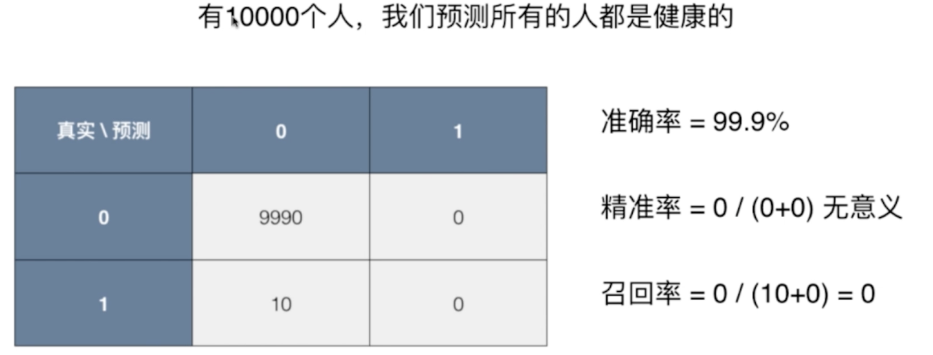
An uncommon disease prediction system, input physical examination information, can judge whether there is a disease;
Prediction accuracy: 99.9%;
If the prevalence rate is 0.1%, our system can achieve 99.9% accuracy in predicting that everyone is healthy.
If the prevalence rate is 0.01%, our system can predict that everyone is healthy, with an accuracy of 99.99%

Conclusion: for extremely skewed data, only using classification accuracy is far from enough.

Solution: use confusion matrix for further analysis

Confusion Matrix

For binary classification problem

• The row represents the true value
• The column represents the predicted value
  • 0 Negative
  • 1 Positive

	0	1
0	TN	FP
1	FN	TP

• TN: True Negative, the predicted negative is correct
• FP: False Positve, predict positive error
• FN: False Negative, negative prediction error
• TP: true positive, the predicted positive is correct

Accuracy and recall

	0	1
0	TN 9978	FP 12
1	FN 2	TP 8

Accuracy

In the forecast data, 100 data are 1. How many are 1.

$ precision = \frac{ TP }{ TP + FP } $

Accuracy in the above data = 8 / (12 + 8) = 40%

When to focus on accuracy?
Such as stock forecast.

recall

Among the predicted data, there are 100 data with 1, and how many 1 are predicted.

$ recall = \frac{ TP }{ TP + FN } $

In the above data, the recall rate = 8 / (2 + 8) = 80%

When to focus on recall?
Such as: disease diagnosis.

At this time, it doesn't matter if the accuracy is a little lower. Can be further diagnosed.

Why?

Why is accuracy and recall better than classification accuracy?

The accuracy of the following cases is meaningless.

F1 Score

F1 will take into account both accuracy and recall, which is the harmonic average of the two (rather than the arithmetic average).

F 1 = 2 ∗ p r e s i c i o n ∗ r e c a l l p r e s i c i o n + r e c a l l F1 = \frac{ 2 * presicion * recall }{ presicion + recall } F1=presicion+recall2∗presicion∗recall​

1 F 1 = 1 2 ( 1 p r e c i s i o n + 1 r e c a l l ) \frac{1}{F1} = \frac{1}{2} ( \frac{1}{ precision } + \frac{1}{ recall } ) F11​=21​(precision1​+recall1​)

Why take the harmonic average?
The harmonic average has a characteristic: if the two are extremely unbalanced, such as one is particularly high and the other is particularly low, F1 will also be very low.

When recall and precision are both 1, F1 takes the maximum value of 1;
F1 is 0 when both are 0.

code implementation

Code implementation of F1

import numpy as np
 
def f1_score(precision, recall):
    try:
        return 2 * precision * recall / (precision + recall)
    except:
        return 0.0
 
# If they are equal, the value of f1 is equal to them
precision = 0.5
recall = 0.5
f1_score(precision, recall)
# 0.5
 
# If the two are different, the result will be pulled down
precision = 0.1
recall = 0.9
f1_score(precision, recall)
# 0.18000000000000002
 
# If one is 0, it will be 0
precision = 0.0
recall = 1.0
f1_score(precision, recall)
# 0.0

Introducing real data

from sklearn import datasets

digits = datasets.load_digits()
X = digits.data
y = digits.target.copy()

y[digits.target==9] = 1
y[digits.target!=9] = 0

 

Confusion matrix, realization of accuracy and recall

def TN(y_true, y_predict):
    assert len(y_true) == len(y_predict)
    return np.sum((y_true == 0) & (y_predict == 0))

def FP(y_true, y_predict):
    assert len(y_true) == len(y_predict)
    return np.sum((y_true == 0) & (y_predict == 1))

def FN(y_true, y_predict):
    assert len(y_true) == len(y_predict)
    return np.sum((y_true == 1) & (y_predict == 0))
    
def TP(y_true, y_predict):
    assert len(y_true) == len(y_predict)
    return np.sum((y_true == 1) & (y_predict == 1))

def confusion_matrix(y_true, y_predict):
    return np.array([
        [TN(y_true, y_predict), FP(y_true, y_predict)],
        [FN(y_true, y_predict), TP(y_true, y_predict)]
    ])

 
def precision_score(y_true, y_predict):
    tp = TP(y_true, y_predict)
    fp = FP(y_true, y_predict)
    try:
        return tp / (tp + fp)
    except:
        return 0.0
        
def recall_score(y_true, y_predict):
    tp = TP(y_true, y_predict)
    fn = FN(y_true, y_predict)
    try:
        return tp / (tp + fn)
    except:
        return 0.0
    
y_log_predict = log_reg.predict(X_test)

TN(y_test, y_log_predict)		# 403
FP(y_test, y_log_predict)		# 2
FN(y_test, y_log_predict)		# 9  
TP(y_test, y_log_predict)		# 36

confusion_matrix(y_test, y_log_predict)
'''
array([[403,   2],
           [  9,  36]])
'''

precision_score(y_test, y_log_predict)	# 0.94736842105263153 

recall_score(y_test, y_log_predict)   # 0.80000000000000004

Confusion matrix in scikit learn, accuracy, recall, F1

from sklearn.model_selection import train_test_split

X_train, X_test, y_train, y_test = train_test_split(X, y, random_state=666)
 
from sklearn.linear_model import LogisticRegression

log_reg = LogisticRegression()
log_reg.fit(X_train, y_train)
log_reg.score(X_test, y_test)
# 0.97555555555555551
 
y_predict = log_reg.predict(X_test)
 
from sklearn.metrics import confusion_matrix, precision_score, recall_score, f1_score

confusion_matrix(y_test, y_predict)  # Confusion matrix
'''
    array([[403,   2],
           [  9,  36]])
'''
 precision_score(y_test, y_predict)
# 0.94736842105263153
 
recall_score(y_test, y_predict)
# 0.80000000000000004
 
f1_score(y_test, y_predict)
# 0.86746987951807231

Balance of precision recall

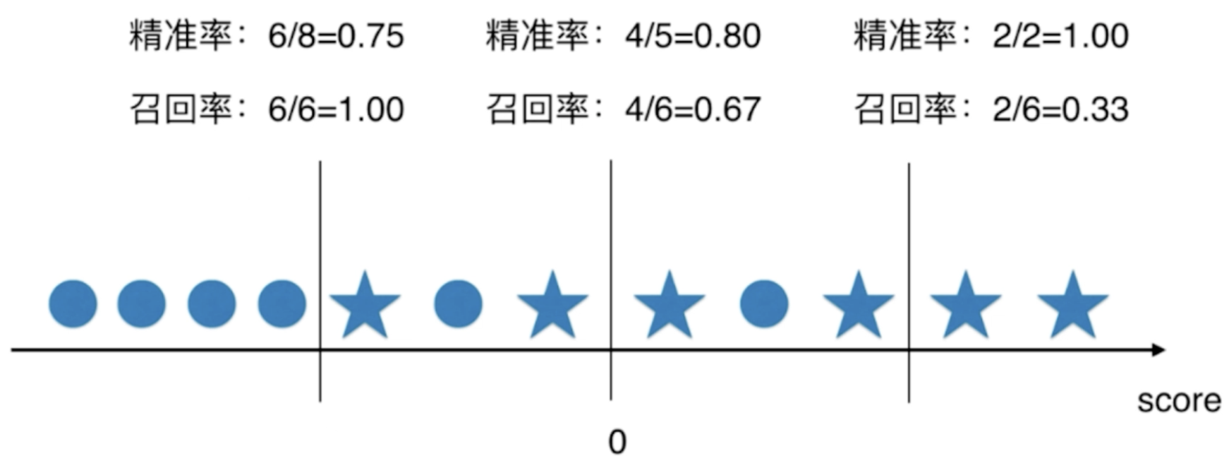
Effect of threshold on accuracy and recall

The star in the figure above is 1;
It can be seen that as the threshold increases, the accuracy rate becomes higher and the recall rate becomes lower;
Precision and precision cannot be contradictory at the same time.

Popular understanding, if you want high accuracy, you need to be particularly sure of the data before marking; But this will miss a lot of samples with a real value of 1.

Code implementation threshold adjustment

# decision_function is a decision-making function. You can know what the corresponding score value is  
  
log_reg.decision_function(X_test)[:10]
# array([-22.05700185, -33.02943631, -16.21335414, -80.37912074, -48.25121102, -24.54004847, -44.39161228, -25.0429358 ,  -0.97827574, -19.71740779])
 
log_reg.predict(X_test)[:10]
# array([0, 0, 0, 0, 0, 0, 0, 0, 0, 0])

 
decision_scores = log_reg.decision_function(X_test)
 
np.min(decision_scores)
# -85.686124167491727
 
np.max(decision_scores)
# 19.889606885682948

Threshold usage 5

y_predict_2 = np.array(decision_scores >= 5, dtype='int')
 
confusion_matrix(y_test, y_predict_2) # array([[404,   1], [ 21,  24]])

 
precision_score(y_test, y_predict_2)	# 0.95999999999999996
 
recall_score(y_test, y_predict_2)  # 0.53333333333333333

Threshold use - 5

y_predict_3 = np.array(decision_scores >= -5, dtype='int')
 
confusion_matrix(y_test, y_predict_3)
# array([[390,  15], [  5,  40]])

 
precision_score(y_test, y_predict_3) # 0.72727272727272729
 
recall_score(y_test, y_predict_3)  #0.88888888888888884

How to select threshold – PR curve

from sklearn.metrics import precision_score
from sklearn.metrics import recall_score

precisions = []
recalls = []

thresholds = np.arange(np.min(decision_scores), np.max(decision_scores), 0.1)

for threshold in thresholds:
    y_predict = np.array(decision_scores >= threshold, dtype='int')
    precisions.append(precision_score(y_test, y_predict))
    recalls.append(recall_score(y_test, y_predict))


plt.plot(thresholds, precisions)
plt.plot(thresholds, recalls)
plt.show()

Precision recall curve

# The x-axis is the accuracy rate and recall is the recall rate; The relationship between the two
plt.plot(precisions, recalls)
plt.show()

Precision recall curve in scikit learn

from sklearn.metrics import precision_recall_curve

precisions, recalls, thresholds = precision_recall_curve(y_test, decision_scores) 
 
# Why 145? The above function will automatically take the most appropriate step size according to the data
precisions.shape	# (145,)  
recalls.shape # (145,)
thresholds.shape  # (144,)
 
plt.plot(thresholds, precisions[:-1])
plt.plot(thresholds, recalls[:-1])
plt.show()

plt.plot(precisions, recalls)
plt.show()

The sharp drop point in the PR curve is likely to be the point where precision and recall reach equilibrium.

The model corresponding to the outer curve is better than the model corresponding to the inner curve;
The description inside is more abstract, and the area of curve package can also be used to describe it.

ROC curve

ROC : Receiver Operation Characteristic Curve
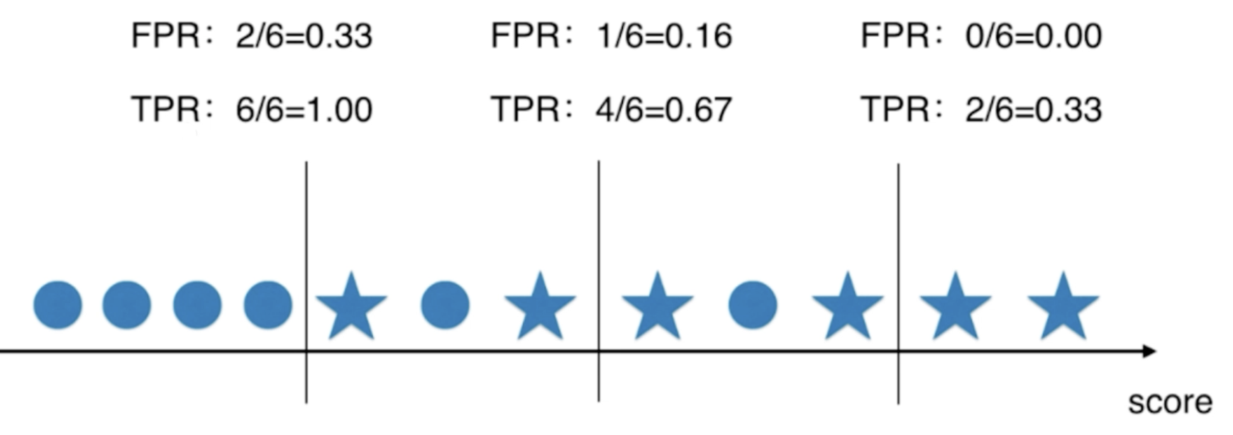
Statistics is commonly used to describe the relationship between TPR and FPR.

TPR is the recall rate, which is predicted to be 1, accounting for 1 of the total
T P R = T P T P + F N TPR = \frac{ TP }{ TP + FN } TPR=TP+FNTP​

FPR: False Position Rate, predicted to be 0, accounting for the proportion of 0 in the total
F P R = F P T N + F P FPR = \frac{ FP }{ TN + FP } FPR=TN+FPFP​

It can be found that TPR and FPR increase with the decrease of threshold; The two trends are consistent;

TPR & fpr code implementation

def TPR(y_true, y_predict):
    tp = TP(y_true, y_predict)
    fn = FN(y_true, y_predict)
    try:
        return tp / (tp + fn)
    except:
        return 0.


def FPR(y_true, y_predict):
    fp = FP(y_true, y_predict)
    tn = TN(y_true, y_predict)
    try:
        return fp / (fp + tn)
    except:
        return 0.
    

ROC code implementation

from playML.metrics import FPR, TPR

fprs = []
tprs = []
thresholds = np.arange(np.min(decision_scores), np.max(decision_scores), 0.1)

for threshold in thresholds:
    y_predict = np.array(decision_scores >= threshold, dtype='int')
    fprs.append(FPR(y_test, y_predict))
    tprs.append(TPR(y_test, y_predict))
 

plt.plot(fprs, tprs)
plt.show()

ROC in scikit learn

from sklearn.metrics import roc_curve

fprs, tprs, thresholds = roc_curve(y_test, decision_scores)
 
plt.plot(fprs, tprs)
plt.show()

ROC AUC

AUC: area under curve

from sklearn.metrics import roc_auc_score

# Calculated area
roc_auc_score(y_test, decision_scores)  # 0.98304526748971188

The model with larger roc area is considered to be a better model.

Implementation of confusion matrix

import matplotlib.pyplot as plt
import itertools

def plot_confusion_matrix(cm, classes,
                          title='Confusion matrix',
                          cmap=plt.cm.Blues):
    """
    This function prints and plots the confusion matrix.
    """
    plt.imshow(cm, interpolation='nearest', cmap=cmap)
    plt.title(title)
    plt.colorbar()
    tick_marks = np.arange(len(classes))
    plt.xticks(tick_marks, classes, rotation=0)
    plt.yticks(tick_marks, classes)

    thresh = cm.max() / 2.
    for i, j in itertools.product(range(cm.shape[0]), range(cm.shape[1])):
        plt.text(j, i, cm[i, j],
                 horizontalalignment="center",
                 color="white" if cm[i, j] > thresh else "black")

    plt.tight_layout()
    plt.ylabel('True label')
    plt.xlabel('Predicted label')

call

from sklearn.metrics import confusion_matrix

LR_model = LogisticRegression()
LR_model = LR_model.fit(X_train, y_train)
y_pred = LR_model.predict(X_test)
cnf_matrix = confusion_matrix(y_test,y_pred)

# recall 
print("Recall metric in the testing dataset: ", cnf_matrix[1,1]/(cnf_matrix[1,0] + cnf_matrix[1,1]))

# accuracy
print("accuracy metric in the testing dataset: ", (cnf_matrix[1,1] + cnf_matrix[0,0])/(cnf_matrix[0,0] + cnf_matrix[1,1]+cnf_matrix[1,0]+cnf_matrix[0,1]))

# Plot non-normalized confusion matrix
class_names = [0,1]
plt.figure()
plot_confusion_matrix(cnf_matrix, classes=class_names, title='Confusion matrix')
plt.show()