1, Experimental description
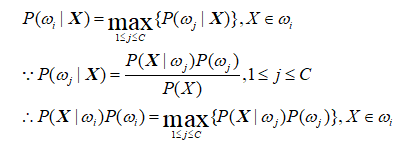
The classification principle of Bayesian classifier is to calculate the posterior probability by using Bayesian formula through the prior probability of an object, that is, the probability that the object belongs to a certain class, and select the class with the maximum posterior probability as the class to which the object belongs. In other words, Bayesian classifier is an optimization in the sense of minimum error rate, which follows the basic principle of "majority dominance".

2, Experimental content
The classification is determined using Bayesian posterior probability:

There are 19 people for physical examination, and the results are shown in the table below. But it was later found that four people forgot to write their gender. Ask, are these four men or women?

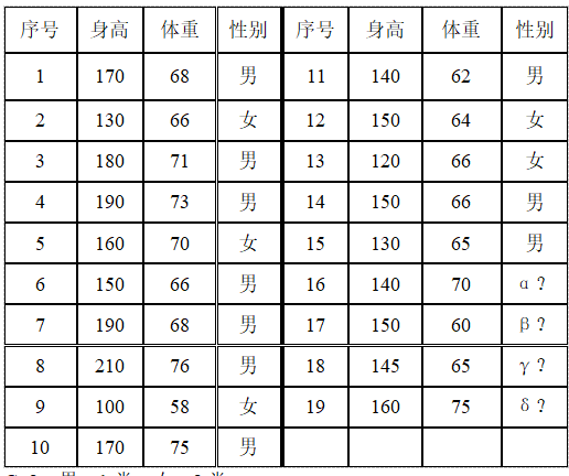
C=2. Male - Category 1, female - Category 2.

3, Bayesian classifier
A Bayesian classifier can simply and naturally represent the above network structure. The classification principle of Bayesian classifier is to calculate the posterior probability by using Bayesian formula through the prior probability of an object, that is, the probability that the object belongs to a certain class, and select the class with the maximum posterior probability as the class to which the object belongs. Under the condition of complete statistical knowledge of patterns, an optimal classifier is designed according to Bayesian decision theory. The classifier is a software or hardware device that assigns a category name to each input mode, and the Bayesian classifier is the classifier with the lowest classification error probability or the lowest average risk at a predetermined cost. Its design method is one of the most basic statistical classification methods.

For Bayesian classifier, the choice of discriminant function is not unique. We can multiply all discriminant functions by the same normal number or add the same constant without affecting the decision result; In a more general case, if each gi (x) is replaced by f(gi (x)), where f(∙) is a monotonically increasing function, the classification effect remains unchanged. Especially for the minimum error rate classification, the same classification results can be obtained by selecting any of the following functions, but some of them are simpler than others.

4, Experimental steps
1. Take the height as an example, draw the histogram of the height of boys and girls and compare them:
The focus here is to read the height of boys and girls from the sample data. xls, record it in the corresponding data, and then display the height frequency of men and women in the histogram.

This program uses the for loop method to read the height and weight of boys and girls into man_h,man_w,woman_h,woman_w. Finally, the hist function is used to display the frequency histogram.

Matlab code:

clear all;
[n,t,r]= xlsread('sample data '); 
l=1;m=1;
for k=1:149 %The sample size is 149
  if n(k,2)==1
    man_h(l)=n(k,4);
    man_w(l)=n(k,5);
    l=l+1;
  else
    woman_h(m)=n(k,4);
    woman_w(m)=n(k,5);
    m=m+1;
  end
end

2. The maximum likelihood estimation method is used to calculate the parameters of height and weight distribution of male and female students
It is assumed that the height and weight of boys and girls obey the normal distribution n( μ,σ^ 2)，
The calculation shows that under the condition of maximum likelihood estimation μ The estimation result is the sample mean, right σ^ 2 the estimation result is sample variance.

%---------The maximum likelihood estimation method is used to calculate the parameters of height and weight distribution of male and female students------------
%Assuming that the height and weight of men and women obey the normal distribution, the estimation result of the mean value by maximum likelihood estimation is the sample mean value, i.e
man_h_u=mean(man_h);woman_h_u=mean(woman_h);        %Average height of men and women
man_w_u=mean(man_w);woman_w_u=mean(woman_w);        %Mean weight of men and women 
man_h_S=0;man_w_S=0;woman_h_S=0;woman_w_S=0;
for m1=1:l-1
    man_h_S=man_h_S+(man_h(m1)-man_h_u)^2;   %Sum of squares of difference between boys' height and mean value
    man_w_S=man_w_S+(man_w(m1)-man_w_u)^2;   %Sum of squares of difference between male weight and mean
end
for w1=1:m-1
    woman_h_S=woman_h_S+(woman_h(w1)-woman_h_u)^2;   %Sum of squares of difference between girls' height and mean value
    woman_w_S=woman_w_S+(woman_w(w1)-woman_w_u)^2;   %Sum of squares of difference between girls' weight and mean value
end 
%The estimation result of the square difference of the maximum likelihood estimation is the sample variance, i.e
sigma1=man_h_S/(l-1);
sigma2=man_w_S/(l-1);
sigma3=woman_h_S/(m-1);
sigma4=woman_w_S/(m-1);  
fprintf('The maximum likelihood estimation mean of boys' height is%f,Variance is%f\n',man_h_u,sigma1);
fprintf('The mean of maximum likelihood estimation of male weight is%f,Variance is%f\n',man_w_u,sigma2);
fprintf('The mean of maximum likelihood estimation of girls' height is%f,Variance is%f\n',woman_h_u,sigma3);
fprintf('The mean value of maximum likelihood estimation of girls' weight is%f,Variance is%f\n',woman_w_u,sigma4); 

3. Bayesian estimation method is used to calculate the parameters of height and weight distribution of male and female students
Firstly, assume that the probability density follows the distribution obtained by the maximum likelihood estimator, that is, P (U1) ~ n (U1, sigma 1 ^ 2),... And set the variance of the a priori distribution of the mean u to be 10:
sigmax1=10; sigmax2 =10; sigmax3 =10; sigmax4 =10;
Bayesian estimation of height and weight of boys and girls was obtained.

<span style="font-size:14px;">%Firstly, it is assumed that the probability density follows the distribution of maximum likelihood estimator, that is p(u1)~N(man_h_u,sigma1)...
%Set mean u The variance of the prior distribution is 10
sigmaX1=10;    
sigmaX2=10;
sigmaX3=10;
sigmaX4=10;

%The Bayesian estimation method is used to calculate the height distribution of men and women in the collective u=uN

%because p(u/X)~N(uN,sigmaN)
%The mean value estimated by Bayesian estimation of minimum error rate is
uN1=(sigma1*sum(man_h)+sigmaX1*man_h_u)/(sigma1*length(man_h)+sigmaX1);
uN2=(sigma2*sum(man_w)+sigmaX2*man_w_u)/(sigma2*length(man_w)+sigmaX2);
uN3=(sigma3*sum(woman_h)+sigmaX3*woman_h_u)/(sigma3*length(woman_h)+sigmaX3);
uN4=(sigma4*sum(woman_w)+sigmaX4*woman_w_u)/(sigma4*length(woman_w)+sigmaX4);

fprintf('Bayesian estimation method is used to calculate the parameters of height and weight distribution of male and female students\n');
fprintf('Set mean u The variance of the prior distribution is 10, i.e sigmaX1=10，sigmaX2=10，sigmaX3=10，sigmaX4=10\n');
fprintf('The mean value estimated by Bayesian estimation of minimum error rate is%f,%f,%f,%f\n',uN1,uN2,uN3,uN4);</span>

4. Bayesian decision with minimum error rate is used to draw the decision surface of category judgment. The height and weight of the samples were (160,45) and (178,70) respectively

--------------Bayesian decision with minimum error rate is used to draw the decision surface of category judgment----------------
%Calculation process of covariance matrix,The main diagonal element is sigma1,sigma2 and sigma3,sigma4,
%Only sub diagonal elements are required sigma12,sigma21 and sigma34,sigma43，And the values of the sub diagonal elements are equal sigma12=sigma21,sigma34=sigma43
%Here, the coefficient is taken as N
C12=0;C34=0;      
for m2=1:length(man_h)
    C12=C12+(man_h(m2)-man_h_u)*(man_w(m2)-man_w_u);   
end
for w2=1:length(woman_h)
    C34=C34+(woman_h(w2)-woman_h_u)*(woman_w(w2)-woman_w_u); 
end
sigma12=C12/m2;
sigma34=C34/w2;
%So the covariance matrix is
sigma_man=[sigma1,sigma12;sigma12,sigma2];   
sigma_woman=[sigma3,sigma34;sigma34,sigma4]; 
%And it is easy to know that the a priori probability is
p_man=m1/(m1+w1);   
p_woman=1-p_man;
syms  x1 x2 %Definition matrix x Two elements of
N_1=[x1-man_h_u,x2-man_w_u];    %(x-u1)
N_2=[x1-woman_h_u,x2-woman_w_u];%(x-u2) 
%The decision surface equation is
g=0.5*N_1*(sigma_man^(-1))*N_1'-0.5*N_2*(sigma_woman^(-1))*N_2'+0.5*log(det(sigma_man)/det(sigma_woman))-log(p_man/p_woman);
%Figure 2 - minimum error rate Bayesian decision category decision surface diagram and sample judgment.
figure(2)
%Figure 2: decision surface
h=ezplot(g,[120,200,20,100]);title('Decision surface function image'),xlabel('height/cm'),ylabel('weight/Kg');
set(h,'Color','r') %Mark the decision face boundary in red
hold on;
%Mark the height and weight data of boys in the sample (blue dot)
for m3=1:l-1
    x=man_h(m3);y=man_w(m3);plot(x,y,'.');
end
%Mark the height and weight data of girls in the sample (magenta dots)
for w3=1:m-1
    x=woman_h(w3);y=woman_w(w3);plot(x,y,'m.');
end
%The height and weight of the samples were determined as follows:(160,45)
x=160;y=45;
plot(x,y,'c*');
%The height and weight of the samples were determined as follows:(178,70)
x=178;y=70;
plot(x,y,'g*'); 
hold off;
grid on;