1, Purpose of the experiment:
1. Deepen the understanding of common indicators of analog filter;
2. Learn the frequency conversion in analog filter;
3. Design the analog filter according to the index requirements and process the signal.
2, Experimental principle:
The design of analog filter is the basis of other filter design, and its design principle is shown in the textbook. The call function of analog filter designed by MATLAB is shown in the textbook. Common function formats are as follows:
1. Butterworth analog filter
[N,wc]=buttord(wp,ws,Ap,As,'s')
[b,a]=butter(N,wc,'ftype','s')
The input parameters wp and ws (rad/s) of the function button represent the passband and stopband cutoff of the filter respectively, and Ap and As (DB) represent the passband and stopband attenuation of the filter‘ S' indicates that the designed filter is an analog filter. The parameter N returned by the function button is the order of the filter, and wc is the 3dB cut-off frequency of BW filter.
The numerator polynomial coefficient (b) and denominator polynomial coefficient (a) of BW filter are obtained by using the function button.
'ftype' indicates the type of filter to be designed. When the filter is designed as low-pass or band-pass filter, this parameter can be defaulted. When ftype=high, the function button obtains the numerator polynomial coefficient (b) and denominator polynomial coefficient (a) of BW high pass filter; When ftype=stop, the function button obtains the numerator polynomial coefficient (b) and denominator polynomial coefficient (a) of BW band stop filter;
Or:
N=buttord(wp,ws,Ap,As,'s'); wc=wp/(10^(0.1*Ap)-1)^(1/2/N); [b,a]=butter(N,wc, 'ftype','s');
Or:
N=buttord(wp,ws,Ap,As,'s'); wc=ws/(10^(0.1*As)-1)^(1/2/N); [b,a]=butter(N,wc, 'ftype','s');
2. Chebyshev type I filter
[N,wc]=cheb1ord(wp,ws,Ap,As,'s');
[b,a]=cheby1(N,Ap,wc, 'ftype','s');
Or,
N=cheb1ord(wp,ws,Ap,As,'s');wc=wp; [b,a]=cheby1(N,Ap,wc, 'ftype','s')
perhaps
N=cheb1ord(wp,ws,Ap,As,'s'); [b,a]=cheby1(N,Ap,wp, 'ftype','s');
3. Chebyshev II filter
[N,wc]=cheb2ord(wp,ws,Ap,As,'s')
[b,a]=cheby2(N,As,wc, 'ftype','s')
perhaps
N=cheb2ord(wp,ws,Ap,As,'s');wc=ws; [b,a]=cheby2(N,As,wc, 'ftype','s')
perhaps
N=cheb2ord(wp,ws,Ap,As,'s'); [b,a]=cheby2(N,As,ws, 'ftype','s')
4. Elliptical filter
[N,wc]=ellipord(wp,ws,Ap,As,'s');
[b,a]=ellip(N,Ap,As,wc, 'ftype','s');
perhaps
N= ellipord (wp,ws,Ap,As,'s');wc=wp; [b,a]=ellip(N,Ap,As,wc, 'ftype','s');
perhaps
N= ellipord (wp,ws,Ap,As,'s'); [b,a]=ellip(N,Ap,As,wp, 'ftype','s');
5. Analog domain frequency conversion
MATLAB provides functions to realize frequency transformation in analog domain, which are:
(1) Analog low pass to high pass conversion
[numt,dent] = lp2hp(num,den,W0)
In high pass, generally W0=1.
(2) Analog low-pass to band-pass conversion
[numt,dent] = lp2bp(num,den,W0,B)
(3) Analog low pass to band stop conversion
[numt,dent] = lp2bs(num,den,W0,B)
Where, num and den respectively represent the numerator polynomial coefficients and denominator polynomial coefficients of the analog low-pass filter system function before the transformation, and W0 and B are the parameters in the transformation. numt and dent respectively represent the numerator polynomial coefficients and denominator polynomial coefficients of the transformed analog filter system function,
6. Supplementary function
(1) The buttap function is used to return the zero, pole and gain of the designed BW filter. The function call format is:
[z,p,k]=buttap(N);
Where Z, P and K are the zeros, poles and gains of the filter system function H (S) respectively, and N is the order of the filter.
(2) cheb1ap function is used to return the zero, pole and gain of the designed CB I filter, and cheb2ap function is used to return the zero, pole and gain of the designed CB II filter. The calling format is:
[z,p,k]= cheb1ap (N,Rp);
[z,p,k]= cheb2ap (N,Rs);
Where Z, P and K are the zeros, poles and gains of the filter system function H (S), N is the order of the filter, Rp is the maximum attenuation value of the filter in the passband, and Rs is the minimum attenuation value of the filter in the stopband.
(3) zp2tf function, the function call format is:
[b,a]=zp2tf (z,p,k);
Where Z, P and K are the zeros, poles and gains of the filter system function H (s), and b and a are the coefficients of the numerator and denominator polynomials of the filter system function H (s), respectively,
(4) freqs function is used to solve the frequency response of analog filter. Its function call format is:
h=freqs(b,a,w);
[h,w]=freqs(b,a,n);
Where, b and a are the coefficients of the numerator and denominator polynomials of the filter system function H (s), w represents the frequency point, n represents the number of points for complex frequency response, and its default value is 512. If the freqs (b,a,w) function is called directly without output parameters, the amplitude frequency response and phase frequency response of the complex frequency response will be drawn directly.
freqs function is used to solve the frequency response of analog filter.
3, Example:
1. Amplitude frequency characteristic curve of BW analog low-pass filter
The procedure is as follows:
clear all
for i=1:4
switch i
    case 1
        N=2;
    case 2
        N=5;
    case 3
        N=10;
    case 4
        N=20;
end
[z,p,k]=buttap(N);
 [b,a]=zp2tf(z,p,k);
 [H,w]=freqs(b,a);
 magH2=(abs(H)).^2;
hold on
plot(w,magH2);
axis([0 2 0 1.1]);
end
xlabel('w/wc');  ylabel('/H(jw)/^2')
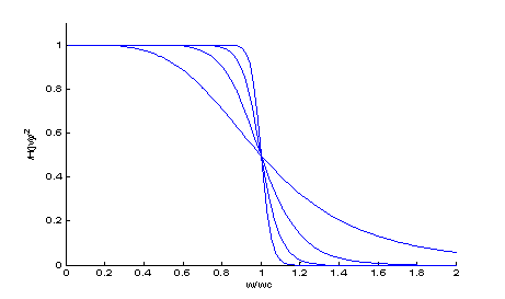
2. (1) a Butterworth analog low-pass filter is designed. The technical indicators are: pass band cutoff 1000Hz, stop band cutoff 1500Hz, pass band ripple 1dB and stop band attenuation 50dB.
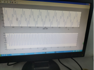
(2) Suppose a signal x (T) = sin(2pif1t)+sin(2pif2t)+sin(2pif3*t), where f1=100Hz, f2=2000Hz, f3=2900Hz, and the sampling frequency of the signal is 10000Hz. The original signal is compared with the analog signal passing through the filter.
clear all
wp=1000 *2*pi;
ws=1500*2*pi;
Ap=1;
As=50;
[N,wc]=buttord(wp,ws,Ap,As,'s'); %Find the minimum order and cut-off frequency of the filter
[b,a]=butter(N,wc,'s');           %Design analog Butterworth filter
w=linspace(0,4000,1000)*2*pi; %Sets the frequency point at which the frequency response is plotted
H=freqs(b,a,w);      % Calculate the complex frequency response of a given frequency point
figure(1)
plot(w/2/pi, 20*log10(abs(H)));
xlabel('frequency/Hz');ylabel('amplitude/dB');
grid on;
% calculation Ap,As

w1=[wp ws];
h=freqs(b,a,w1);
fprintf('Ap=%.4f\n',-20*log10(abs(h(1))));
fprintf('As=%.4f\n',-20*log10(abs(h(2))));

fs=10000;
dt=1/fs;   %Analog signal sampling interval
f1=100;f2=2000;f3=2900;
t=0:dt:0.1;
x=sin(2*pi*f1*t)+sin(2*pi*f2*t)+sin(2*pi*f3*t);
H=[tf(b,a)];  %Filter in MATLAB Representation in
y=lsim(H,x,t); % Analog output
figure(2)
subplot(2,1,1)
plot(t,x);
xlabel ('(a)Input signal');
subplot(2,1,2)
plot(t,y);
xlabel('(b)output signal');
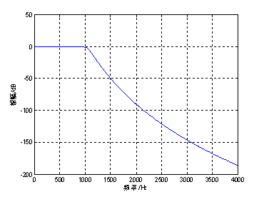
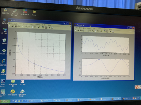
Figure 1 amplitude response function of analog low-pass filter
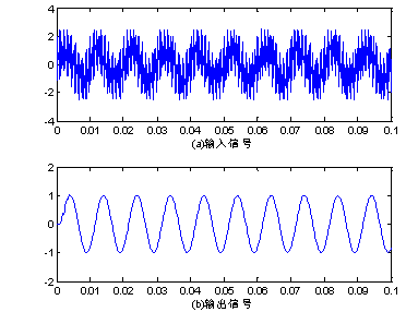
Fig. 2 input-output function of filter
Ap=0.9053; As=50.0000
2. Design a Butterworth analog bandpass filter. The technical indexes are: passband frequency: 1000-2000Hz, transition bandwidth on both sides: 500Hz, passband ripple: 1dB, stopband attenuation: 100dB.
Method 1:
clear all
wp1=1000*2*pi;
wp2=2000*2*pi;
ws1=500*2*pi;
ws2=2500*2*pi;
B=wp2-wp1;
W0=sqrt(wp1*wp2);
Ap=1;
As=100;
ws11=(ws1^2-W0^2)/(B*ws1);     %Bandpass to lowpass frequency conversion
ws22=(ws2^2-W0^2)/(B*ws2);
wp=1;
ws=min(abs(ws11),abs(ws22));    %Stopband cut-off of low-pass filter
[N,wc]=buttord(wp,ws,Ap,As,'s'); %Find the minimum order and cut-off frequency of the filter
[b,a]=butter(N,wc,'s');           %Design analog Butterworth filter
[c,d]=lp2bp(b,a,W0,B);    %Convert low-pass to band-pass
w=linspace(1,3000,1000)*2*pi; %Sets the frequency point at which the frequency response is plotted
H=freqs(c,d,w);      % Calculate the complex frequency response of a given frequency point
plot(w/2/pi,abs(H));
xlabel('frequency/Hz');ylabel('amplitude/dB');
grid on;
% calculation Ap,As
w1=[wp1 wp2 ws1 ws2];
h=freqs(c,d,w1);
fprintf('Ap1=%.4f\n',-20*log10(abs(h(1))));
fprintf('Ap2=%.4f\n',-20*log10(abs(h(2))));
fprintf('As1=%.4f\n',-20*log10(abs(h(3))));
fprintf('As1=%.4f\n',-20*log10(abs(h(4))));
Operation results:
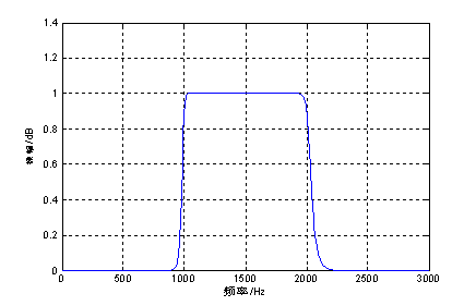
Fig. 3 amplitude response function of bandpass filter
Ap1=0.9713;Ap2=0.9716;As1=244.2668;As1=100.0000
Method 2:
The procedure is as follows:
clear all
wp=[1000 2000]*2*pi;
ws=[500 2500]*2*pi;
Ap=1;
As=100;
[N,wc]=buttord(wp,ws,Ap,As,'s'); %Find the minimum order and cut-off frequency of the filter
[b,a]=butter(N,wc,'s');           %Design analog Butterworth filter
w=linspace(1,3000,1000)*2*pi; %Sets the frequency point at which the frequency response is plotted
H=freqs(b,a,w);      % Calculate the complex frequency response of a given frequency point
plot(w/2/pi,abs(H));
xlabel('frequency/Hz');ylabel('amplitude/dB');
grid on;
% calculation Ap,As
w1=[wp ws];
h=freqs(b,a,w1);
fprintf('Ap1=%.4f\n',-20*log10(abs(h(1))));
fprintf('Ap2=%.4f\n',-20*log10(abs(h(2))));
fprintf('As1=%.4f\n',-20*log10(abs(h(3))));
fprintf('As1=%.4f\n',-20*log10(abs(h(4))));
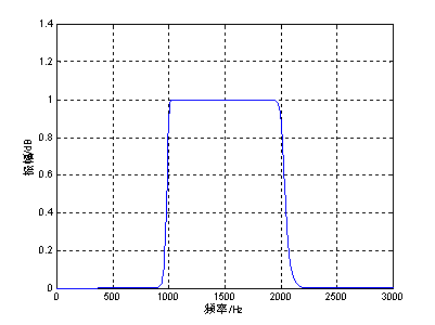
Fig. 3 amplitude response function of bandpass filter
Ap1=0.9724;Ap2=0.9721;As1=244.2646;As1=99.9998
4, Job:
1. Suppose a signal x (T) = sin(2pif1t)+0.5cos(2pif2t), where f1=20Hz and f2=100Hz.
(1) Please design an analog filter to filter out f2. Please write the program and draw the graph of the original signal and the output signal of the original signal through the filter.
clear all
wp=52*2*pi;
ws=80*2*pi;
Ap=1;
As=50;
[N,wc]=buttord(wp,ws,Ap,As,'s'); %Find the minimum order and cut-off frequency of the filter
[b,a]=butter(N,wc,'s');           %Design analog Butterworth filter
w=linspace(0,500,1000)*2*pi; %Sets the frequency point at which the frequency response is plotted
H=freqs(b,a,w);      % Calculate the complex frequency response of a given frequency point
figure(1)
plot(w/2/pi, 20*log10(abs(H)));
xlabel('frequency/Hz');ylabel('amplitude/dB');
grid on;
% calculation Ap,As

w1=[wp ws];
h=freqs(b,a,w1);
fprintf('Ap=%.4f\n',-20*log10(abs(h(1))));
fprintf('As=%.4f\n',-20*log10(abs(h(2))));

fs=10000;
dt=1/fs;   %Analog signal sampling interval
f1=20;f2=100;
t=0:dt:0.1;
x=sin(2*pi*f1*t)+0.5*cos(2*pi*f2*t);
H=[tf(b,a)];  %Filter in MATLAB Representation in
y=lsim(H,x,t); % Analog output
figure(2)
subplot(2,1,1)
plot(t,x);
xlabel ('(a)Input signal');
subplot(2,1,2)
plot(t,y);
xlabel('(b)output signal');
(2) Please design an analog filter to filter out f1. Please write the program and draw the graph of the original signal and the output signal of the original signal through the filter.
2. Suppose a signal x (T) = sin(2pif1t)+sin(2pif2t)+sin(2pif3*t), where f1=200Hz, f2=1500Hz, f3=2900Hz, and the sampling frequency of the signal is 10000Hz.
(1) Please design an analog filter to keep f2 and filter out f1 and f3.
clear all
wp1=1000*2*pi;
wp2=2000*2*pi;
ws1=500*2*pi;
ws2=2500*2*pi;
B=wp2-wp1;
W0=sqrt(wp1*wp2);
Ap=1;
As=100;
ws11=(ws1^2-W0^2)/(B*ws1);     %Bandpass to lowpass frequency conversion
ws22=(ws2^2-W0^2)/(B*ws2);
wp=1;
ws=min(abs(ws11),abs(ws22));    %Stopband cut-off of low-pass filter
[N,wc]=buttord(wp,ws,Ap,As,'s'); %Find the minimum order and cut-off frequency of the filter
[b,a]=butter(N,wc,'s');           %Design analog Butterworth filter
[c,d]=lp2bp(b,a,W0,B);    %Convert low-pass to band-pass
w=linspace(1,3000,1000)*2*pi; %Sets the frequency point at which the frequency response is plotted
H=freqs(c,d,w);      % Calculate the complex frequency response of a given frequency point
plot(w/2/pi,abs(H));
xlabel('frequency/Hz');ylabel('amplitude/dB');
grid on;
% calculation Ap,As
w1=[wp1 wp2 ws1 ws2];
h=freqs(c,d,w1);
fprintf('Ap1=%.4f\n',-20*log10(abs(h(1))));
fprintf('Ap2=%.4f\n',-20*log10(abs(h(2))));
fprintf('As1=%.4f\n',-20*log10(abs(h(3))));
fprintf('As1=%.4f\n',-20*log10(abs(h(4))));

(2) Please design an analog filter to filter out f2 and keep f1 and f3.
More relevant articles can be found here
Digital signal processing -- full set of Matlab experimental report