This article is shared from Huawei cloud community< [Python artificial intelligence] 21 Detailed explanation of Word2Vec+CNN Chinese text classification and comparison with machine learning algorithm >, by eastmount.
I Text classification
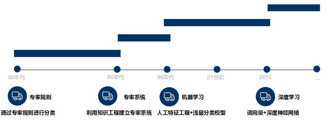
Text classification aims to automatically classify and mark the text set according to a certain classification system or standard. It belongs to an automatic classification based on the classification system. Text classification can be traced back to the 1950s, when text classification was mainly carried out through expert defined rules; In the 1980s, the expert system established by knowledge engineering appeared; In the 1990s, text classification was carried out through artificial feature engineering and shallow classification model with the help of machine learning method. At present, word vector and deep neural network are mostly used for text classification.
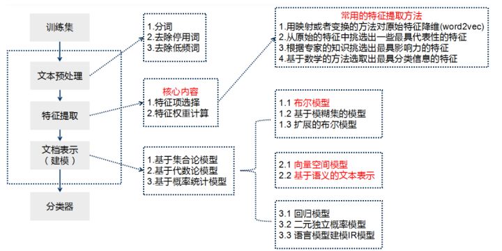
Teacher Niu Yafeng summarized the traditional text classification process as shown in the figure below. In the traditional text classification, most machine learning methods are basically applied in the field of text classification. It mainly includes:
- Naive Bayes
- KNN
- SVM
- Random forest \ decision tree
- Collection class method
- Maximum entropy
- neural network
The basic process of text classification using Keras framework is as follows:
- Step 1: text preprocessing, word segmentation - > remove stop words - > statistics, select top n words as feature words
- Step 2: generate ID for each feature word
- Step 3: convert the text into ID sequence and fill in the left
- Step 4: shuffle the training set
- Step 5: Embedding Layer converts words into word vectors
- Step 6: add model and construct neural network structure
- Step 7: Training Model
- Step 8: get the accuracy, recall and F1 value
Note that if TFIDF is used instead of word vector for document representation, the TFIDF matrix is generated after word segmentation and stop, and then the model is input. This paper will use word vector and TFIDF to experiment.
In Mr. Zhihu Shi's“ https://zhuanlan.zhihu.com/p/34212945 ”In summary, there are five major categories of text classification based on deep learning:
- Word embedding vectorization: word2vec, FastText, etc
- Convolutional neural network feature extraction: TextCNN, char CNN, etc
- Context mechanism: TextRNN (cyclic neural network), BiRNN, BiLSTM, RCNN, TextRCNN(TextRNN+CNN), etc
- Memory storage mechanism: EntNet, DMN, etc
- Attention mechanism: HAN, TextRNN+Attention, etc
II Text classification based on random forest
This part mainly focuses on common text classification cases. Due to the good effect of random forest, this method is mainly shared. The specific steps include:
- Read CSV Chinese text
- Call Jieba library to realize Chinese word segmentation and data cleaning
- Feature extraction is represented by TF-IDF or Word2Vec word vector
- Classification based on machine learning
- Calculation and evaluation of accuracy, recall and F value
1. Text classification
(1). data set
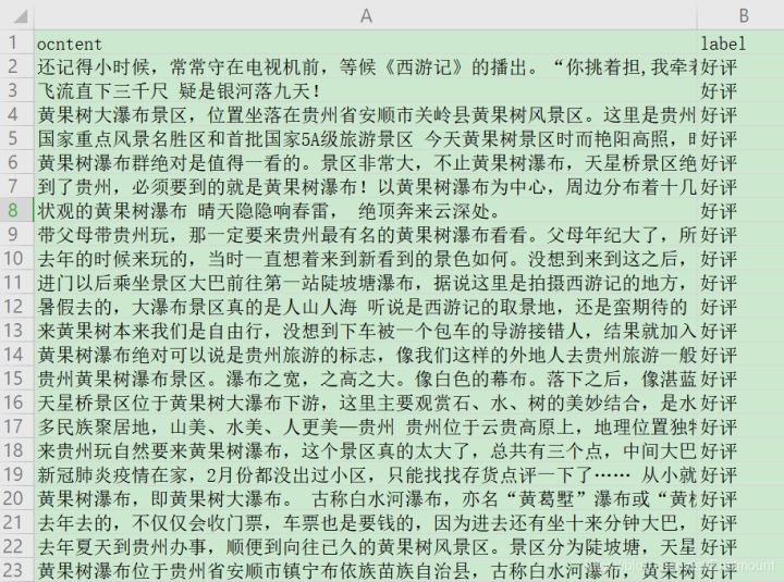
The data in this paper is the recent tourism review text of Huangguoshu waterfall in Guizhou. It comes from dianping.com, with a total of 240 data, including 114 bad evaluation data and 126 good evaluation data, as shown in the figure below:
(2) Random forest text classification
This article will not describe the code implementation process in detail. Many previous articles have introduced it, and the source code has detailed comments for your reference.
# -*- coding:utf-8 -*-
import csv
import numpy as np
import jieba
import jieba.analyse
from sklearn import feature_extraction
from sklearn.feature_extraction.text import TfidfVectorizer
from sklearn.feature_extraction.text import CountVectorizer
from sklearn.feature_extraction.text import TfidfTransformer
from sklearn.model_selection import train_test_split
from sklearn.metrics import classification_report
from sklearn.ensemble import RandomForestClassifier
#----------------------------------Step 1: read the file--------------------------------
file = "data.csv"
with open(file, "r", encoding="UTF-8") as f:
# Using CSV Dictreader reads the information in the file
reader = csv.DictReader(f)
labels = []
contents = []
for row in reader:
# Data element acquisition
if row['label'] == 'Praise':
res = 0
else:
res = 1
labels.append(res)
content = row['content']
seglist = jieba.cut(content,cut_all=False) #Precise mode
output = ' '.join(list(seglist)) #Space splicing
#print(output)
contents.append(output)
print(labels[:5])
print(contents[:5])
#----------------------------------Step 2 data preprocessing--------------------------------
# Convert the words in the text into word frequency matrix. The matrix element a[i][j] represents the word frequency of j words under class I text
vectorizer = CountVectorizer()
# This class will count the TF IDF weight of each word
transformer = TfidfTransformer()
#First fit_transform is the second fit to calculate TF IDF_ Transform is to convert text into word frequency matrix
tfidf = transformer.fit_transform(vectorizer.fit_transform(contents))
for n in tfidf[:5]:
print(n)
#tfidf = tfidf.astype(np.float32)
print(type(tfidf))
# Get all words in the word bag model
word = vectorizer.get_feature_names()
for n in word[:5]:
print(n)
print("Number of words:", len(word))
# The TF IDF matrix is extracted, and the element w[i][j] represents the TF IDF weight of j words in class I text
X = tfidf.toarray()
print(X.shape)
# Using train_test_split split X y list
# X_ The number of train matrices corresponds to y_ Number of train lists (one-to-one correspondence) - > > used to train models
# X_ Corresponding to the number of test matrices (one-to-one correspondence) - > > used to test the accuracy of the model
X_train, X_test, y_train, y_test = train_test_split(X, labels, test_size=0.3, random_state=1)
#----------------------------------Step 3 machine learning classification--------------------------------
# Random forest classification method model
# n_estimators: the number of trees in the forest
clf = RandomForestClassifier(n_estimators=20)
# Training model
clf.fit(X_train, y_train)
# The accuracy of the model is calculated using the test values
print('Accuracy of model:{}'.format(clf.score(X_test, y_test)))
print("\n")
# Prediction results
pre = clf.predict(X_test)
print('Prediction results:', pre[:10])
print(len(pre), len(y_test))
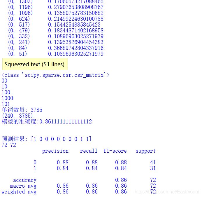
print(classification_report(y_test, pre))The output results are shown in the figure below. The average accuracy rate of random forest is 0.86, the recall rate is 0.86, and the F value is also 0.86.
2. Algorithm evaluation
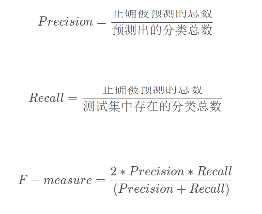
Next, the author tries to customize the accuracy, Recall and F-measure. The calculation formula is as follows:
This paper is mainly divided into two categories: 1 and 2
# -*- coding:utf-8 -*-
import csv
import numpy as np
import jieba
import jieba.analyse
from sklearn import feature_extraction
from sklearn.feature_extraction.text import TfidfVectorizer
from sklearn.feature_extraction.text import CountVectorizer
from sklearn.feature_extraction.text import TfidfTransformer
from sklearn.model_selection import train_test_split
from sklearn.metrics import classification_report
from sklearn.ensemble import RandomForestClassifier
#----------------------------------Step 1: read the file--------------------------------
file = "data.csv"
with open(file, "r", encoding="UTF-8") as f:
# Using CSV Dictreader reads the information in the file
reader = csv.DictReader(f)
labels = []
contents = []
for row in reader:
# Data element acquisition
if row['label'] == 'Praise':
res = 0
else:
res = 1
labels.append(res)
content = row['content']
seglist = jieba.cut(content,cut_all=False) #Precise mode
output = ' '.join(list(seglist)) #Space splicing
#print(output)
contents.append(output)
print(labels[:5])
print(contents[:5])
#----------------------------------Step 2 data preprocessing--------------------------------
# Convert the words in the text into word frequency matrix. The matrix element a[i][j] represents the word frequency of j words under class I text
vectorizer = CountVectorizer()
# This class will count the TF IDF weight of each word
transformer = TfidfTransformer()
#First fit_transform is the second fit to calculate TF IDF_ Transform is to convert text into word frequency matrix
tfidf = transformer.fit_transform(vectorizer.fit_transform(contents))
for n in tfidf[:5]:
print(n)
#tfidf = tfidf.astype(np.float32)
print(type(tfidf))
# Get all words in the word bag model
word = vectorizer.get_feature_names()
for n in word[:5]:
print(n)
print("Number of words:", len(word))
# The TF IDF matrix is extracted, and the element w[i][j] represents the TF IDF weight of j words in class I text
X = tfidf.toarray()
print(X.shape)
# Using train_test_split split X y list
# X_ The number of train matrices corresponds to y_ Number of train lists (one-to-one correspondence) - > > used to train models
# X_ Corresponding to the number of test matrices (one-to-one correspondence) - > > used to test the accuracy of the model
X_train, X_test, y_train, y_test = train_test_split(X, labels, test_size=0.3, random_state=1)
#----------------------------------Step 3 machine learning classification--------------------------------
# Random forest classification method model
# n_estimators: the number of trees in the forest
clf = RandomForestClassifier(n_estimators=20)
# Training model
clf.fit(X_train, y_train)
# The accuracy of the model is calculated using the test values
print('Accuracy of model:{}'.format(clf.score(X_test, y_test)))
print("\n")
# Prediction results
pre = clf.predict(X_test)
print('Prediction results:', pre[:10])
print(len(pre), len(y_test))
print(classification_report(y_test, pre))
#----------------------------------Step 4 evaluation results--------------------------------
def classification_pj(name, y_test, pre):
print("Algorithm evaluation:", name)
# Accuracy = total number of individuals correctly identified / total number of individuals identified
# Recall = total number of correctly identified individuals / total number of individuals in the test set
# F value F-measure = accuracy * recall * 2 / (accuracy + recall)
YC_B, YC_G = 0,0 #Predict bad good
ZQ_B, ZQ_G = 0,0 #correct
CZ_B, CZ_G = 0,0 #existence
#0-good 1-bad is calculated at the same time to prevent the change of class standard
i = 0
while i<len(pre):
z = int(y_test[i]) #real
y = int(pre[i]) #forecast
if z==0:
CZ_G += 1
else:
CZ_B += 1
if y==0:
YC_G += 1
else:
YC_B += 1
if z==y and z==0 and y==0:
ZQ_G += 1
elif z==y and z==1 and y==1:
ZQ_B += 1
i = i + 1
print(ZQ_B, ZQ_G, YC_B, YC_G, CZ_B, CZ_G)
print("")
# Result output
P_G = ZQ_G * 1.0 / YC_G
P_B = ZQ_B * 1.0 / YC_B
print("Precision Good 0:", P_G)
print("Precision Bad 1:", P_B)
R_G = ZQ_G * 1.0 / CZ_G
R_B = ZQ_B * 1.0 / CZ_B
print("Recall Good 0:", R_G)
print("Recall Bad 1:", R_B)
F_G = 2 * P_G * R_G / (P_G + R_G)
F_B = 2 * P_B * R_B / (P_B + R_B)
print("F-measure Good 0:", F_G)
print("F-measure Bad 1:", F_B)
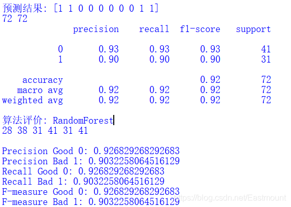
# function call
classification_pj("RandomForest", y_test, pre)The output results are shown in the figure below, in which the accuracy, recall and F values of high praise are 0.9268, 0.9268 and 0.9268 respectively, and the accuracy, recall and F values of poor evaluation are 0.9032, 0.9032 and 0.9032 respectively.
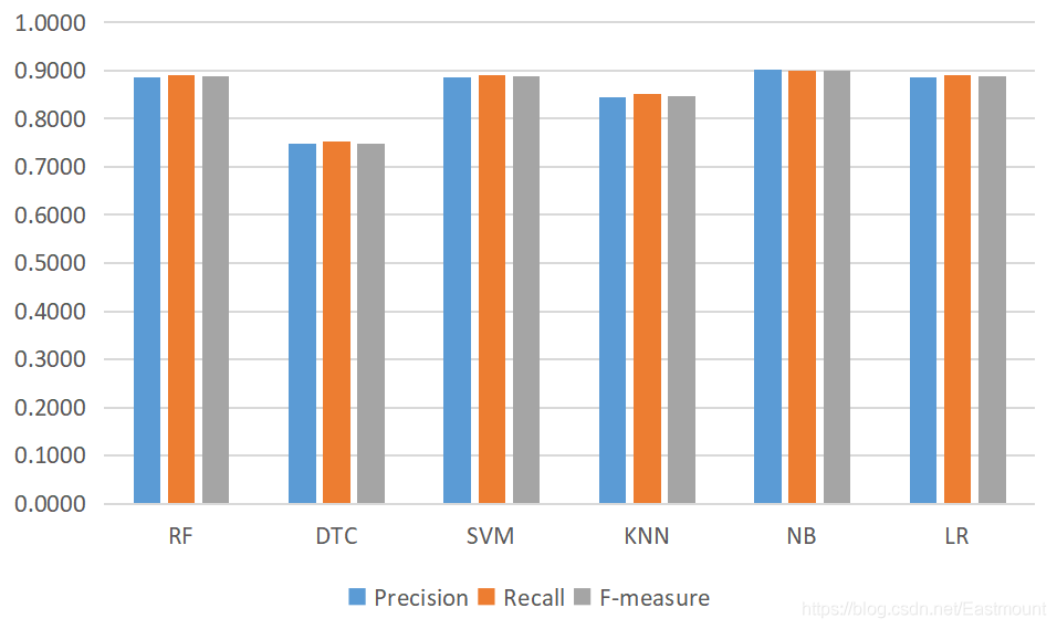
3. Algorithm comparison
Finally, the author gives the text classification results of machine learning RF, DTC, SVM, KNN, NB and LR, which is also a very common operation in writing papers.
# -*- coding:utf-8 -*-
import csv
import numpy as np
import jieba
import jieba.analyse
from sklearn import feature_extraction
from sklearn.feature_extraction.text import TfidfVectorizer
from sklearn.feature_extraction.text import CountVectorizer
from sklearn.feature_extraction.text import TfidfTransformer
from sklearn.model_selection import train_test_split
from sklearn.metrics import classification_report
from sklearn.ensemble import RandomForestClassifier
from sklearn.tree import DecisionTreeClassifier
from sklearn import svm
from sklearn import neighbors
from sklearn.naive_bayes import MultinomialNB
from sklearn.linear_model import LogisticRegression

#----------------------------------Step 1: read the file--------------------------------
file = "data.csv"

with open(file, "r", encoding="UTF-8") as f:
    # Using CSV Dictreader reads the information in the file
    reader = csv.DictReader(f)
    labels = []
    contents = []
    for row in reader:
        # Data element acquisition
        if row['label'] == 'Praise':
            res = 0
        else:
            res = 1
        labels.append(res)
        content = row['content']
        seglist = jieba.cut(content,cut_all=False)  #Precise mode
        output = ' '.join(list(seglist))            #Space splicing
        #print(output)
        contents.append(output)

print(labels[:5])
print(contents[:5])

#----------------------------------Step 2 data preprocessing--------------------------------
# Convert the words in the text into word frequency matrix. The matrix element a[i][j] represents the word frequency of j words under class I text
vectorizer = CountVectorizer()

# This class will count the TF IDF weight of each word
transformer = TfidfTransformer()

#First fit_transform is the second fit to calculate TF IDF_ Transform is to convert text into word frequency matrix
tfidf = transformer.fit_transform(vectorizer.fit_transform(contents))
for n in tfidf[:5]:
    print(n)
#tfidf = tfidf.astype(np.float32)
print(type(tfidf))

# Get all words in the word bag model
word = vectorizer.get_feature_names()
for n in word[:5]:
    print(n)
print("Number of words:", len(word))

# The TF IDF matrix is extracted, and the element w[i][j] represents the TF IDF weight of j words in class I text
X = tfidf.toarray()
print(X.shape)

# Using train_test_split split X y list
# X_ The number of train matrices corresponds to y_ Number of train lists (one-to-one correspondence) - > > used to train models
# X_ Corresponding to the number of test matrices 	  (one-to-one correspondence) - > > used to test the accuracy of the model
X_train, X_test, y_train, y_test = train_test_split(X, labels, test_size=0.3, random_state=1)

#----------------------------------Step 4 evaluation results--------------------------------
def classification_pj(name, y_test, pre):
    print("Algorithm evaluation:", name)

    # Accuracy = total number of individuals correctly identified / total number of individuals identified
    # Recall = total number of correctly identified individuals / total number of individuals in the test set
    # F value F-measure = accuracy * recall * 2 / (accuracy + recall)

    YC_B, YC_G = 0,0  #Predict bad good
    ZQ_B, ZQ_G = 0,0  #correct
    CZ_B, CZ_G = 0,0  #existence

    #0-good 1-bad is calculated at the same time to prevent the change of class standard
    i = 0
    while i<len(pre):
        z = int(y_test[i])   #real
        y = int(pre[i])      #forecast

        if z==0:
            CZ_G += 1
        else:
            CZ_B += 1

        if y==0:
            YC_G += 1
        else:
            YC_B += 1

        if z==y and z==0 and y==0:
            ZQ_G += 1
        elif z==y and z==1 and y==1:
            ZQ_B += 1
        i = i + 1
    print(ZQ_B, ZQ_G, YC_B, YC_G, CZ_B, CZ_G)

    # Result output
    P_G = ZQ_G * 1.0 / YC_G
    P_B = ZQ_B * 1.0 / YC_B
    print("Precision Good 0:{:.4f}".format(P_G))
    print("Precision Bad 1:{:.4f}".format(P_B))
    print("Avg_precision:{:.4f}".format((P_G+P_B)/2))

    R_G = ZQ_G * 1.0 / CZ_G
    R_B = ZQ_B * 1.0 / CZ_B
    print("Recall Good 0:{:.4f}".format(R_G))
    print("Recall Bad 1:{:.4f}".format(R_B))
    print("Avg_recall:{:.4f}".format((R_G+R_B)/2))

    F_G = 2 * P_G * R_G / (P_G + R_G)
    F_B = 2 * P_B * R_B / (P_B + R_B)
    print("F-measure Good 0:{:.4f}".format(F_G))
    print("F-measure Bad 1:{:.4f}".format(F_B))
    print("Avg_fmeasure:{:.4f}".format((F_G+F_B)/2))

#----------------------------------Step 3 machine learning classification--------------------------------
# Random forest classification method model
rf = RandomForestClassifier(n_estimators=20)
rf.fit(X_train, y_train)
pre = rf.predict(X_test)
print("Random forest classification")
print(classification_report(y_test, pre))
classification_pj("RandomForest", y_test, pre)
print("\n")

# Decision tree classification method model
dtc = DecisionTreeClassifier()
dtc.fit(X_train, y_train)
pre = dtc.predict(X_test)
print("Decision tree classification")
print(classification_report(y_test, pre))
classification_pj("DecisionTree", y_test, pre)
print("\n")

# SVM classification method model
SVM = svm.LinearSVC() #Support vector machine classifier LinearSVC
SVM.fit(X_train, y_train)
pre = SVM.predict(X_test)
print("Support vector machine classification")
print(classification_report(y_test, pre))
classification_pj("LinearSVC", y_test, pre)
print("\n")

# KNN classification method model
knn = neighbors.KNeighborsClassifier() #n_neighbors=11
knn.fit(X_train, y_train)
pre = knn.predict(X_test)
print("Nearest neighbor classification")
print(classification_report(y_test, pre))
classification_pj("KNeighbors", y_test, pre)
print("\n")

# Naive Bayesian classification method model
nb = MultinomialNB()
nb.fit(X_train, y_train)
pre = nb.predict(X_test)
print("naive bayesian classification ")
print(classification_report(y_test, pre))
classification_pj("MultinomialNB", y_test, pre)
print("\n")

# Logistic regression classification method model
LR = LogisticRegression(solver='liblinear')
LR.fit(X_train, y_train)
pre = LR.predict(X_test)
print("Logistic regression classification")
print(classification_report(y_test, pre))
classification_pj("LogisticRegression", y_test, pre)
print("\n")
The output results are as follows. It is found that the effect of Bayesian algorithm in text classification is still great; At the same time, the effects of random forest, logistic regression and SVM are all good.
The complete results are as follows:
Random forest classification
              precision    recall  f1-score   support

           0       0.92      0.88      0.90        41
           1       0.85      0.90      0.88        31

    accuracy                           0.89        72
   macro avg       0.89      0.89      0.89        72
weighted avg       0.89      0.89      0.89        72

Algorithm evaluation: RandomForest
28 36 33 39 31 41
Precision Good 0:0.9231
Precision Bad 1:0.8485
Avg_precision:0.8858
Recall Good 0:0.8780
Recall Bad 1:0.9032
Avg_recall:0.8906
F-measure Good 0:0.9000
F-measure Bad 1:0.8750
Avg_fmeasure:0.8875
Decision tree classification
              precision    recall  f1-score   support

           0       0.81      0.73      0.77        41
           1       0.69      0.77      0.73        31

    accuracy                           0.75        72
   macro avg       0.75      0.75      0.75        72
weighted avg       0.76      0.75      0.75        72

Algorithm evaluation: DecisionTree
24 30 35 37 31 41
Precision Good 0:0.8108
Precision Bad 1:0.6857
Avg_precision:0.7483
Recall Good 0:0.7317
Recall Bad 1:0.7742
Avg_recall:0.7530
F-measure Good 0:0.7692
F-measure Bad 1:0.7273
Avg_fmeasure:0.7483
Support vector machine classification
Nearest neighbor classification
naive bayesian classification
Logistic regression classification
......
III Text classification based on CNN
As long as there are many CNN methods in the field of text analysis, we can start to apply them to the field of text analysis. Here only the most basic and available methods and source code are given, hoping to help you.
1. Data preprocessing
In the last part, when I was writing machine learning text classification, I already introduced Chinese word segmentation and other preprocessing operations. Why should I introduce this part? Because here I want to add two new operations:
- De stop word
- Part of speech tagging
These two operations are very important in the process of text mining. On the one hand, they can improve our classification effect, on the other hand, they can filter out irrelevant feature words, and part of speech tagging can also assist us in other analysis, such as emotion analysis, public opinion mining and so on.
The code of this part is as follows:
# -*- coding:utf-8 -*-
import csv
import numpy as np
import jieba
import jieba.analyse
import jieba.posseg as pseg
from sklearn import feature_extraction
from sklearn.feature_extraction.text import TfidfVectorizer
from sklearn.feature_extraction.text import CountVectorizer
from sklearn.feature_extraction.text import TfidfTransformer
from sklearn.model_selection import train_test_split
from sklearn.metrics import classification_report
#----------------------------------Step 1 data preprocessing--------------------------------
file = "data.csv"
# Get stop words
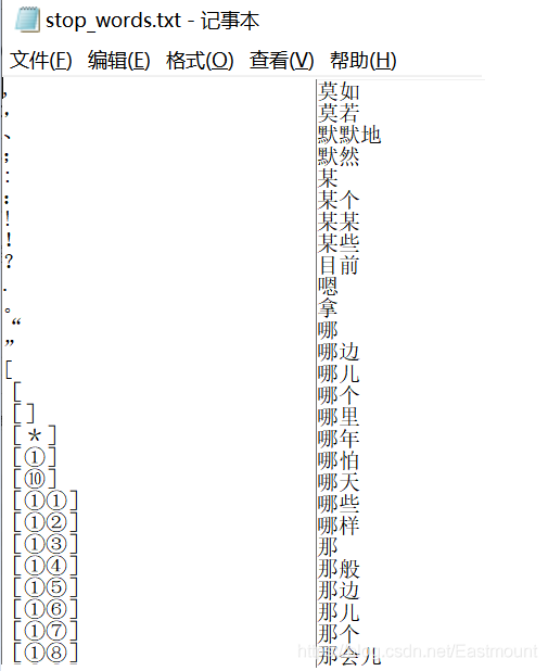
def stopwordslist(): #Load stop list
stopwords = [line.strip() for line in open('stop_words.txt', encoding="UTF-8").readlines()]
return stopwords
# Remove stop words
def deleteStop(sentence):
stopwords = stopwordslist()
outstr = ""
for i in sentence:
# print(i)
if i not in stopwords and i!="\n":
outstr += i
return outstr
# Chinese word segmentation
Mat = []
with open(file, "r", encoding="UTF-8") as f:
# Using CSV Dictreader reads the information in the file
reader = csv.DictReader(f)
labels = []
contents = []
for row in reader:
# Data element acquisition
if row['label'] == 'Praise':
res = 0
else:
res = 1
labels.append(res)
# Chinese word segmentation
content = row['content']
#print(content)
seglist = jieba.cut(content,cut_all=False) #Precise mode
#print(seglist)
# De stop word
stc = deleteStop(seglist) #Note that there are no spaces in the sentence
# Space splicing
seg_list = jieba.cut(stc,cut_all=False)
output = ' '.join(list(seg_list))
#print(output)
contents.append(output)
# Part of speech tagging
res = pseg.cut(stc)
seten = []
for word,flag in res:
if flag not in ['nr','ns','nt','mz','m','f','ul','l','r','t']:
seten.append(word)
Mat.append(seten)
print(labels[:5])
print(contents[:5])
print(Mat[:5])
# File write
fileDic = open('wordCut.txt', 'w', encoding="UTF-8")
for i in Mat:
fileDic.write(" ".join(i))
fileDic.write('\n')
fileDic.close()
words = [line.strip().split(" ") for line in open('WordCut.txt',encoding='UTF-8').readlines()]
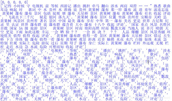
print(words[:5])The running results are shown in the figure below. It can be seen that the original text is segmented, and the stop words such as "Huan", "often" are filtered out and presented in two forms. Readers can conduct follow-up analysis in combination with their own needs. At the same time, the text after word segmentation is also written into wordcut Txt file.
- contents: displays sentences that have been segmented and exist in the form of a list
- Mat: displays word sequences that have been segmented and exist in the form of a list

2. Feature extraction and Word2Vec word vector conversion
(1) Feature word number
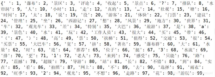
First, we call Tokenizer and fit_ on_ The texts function numbers each word in the text. The higher the word frequency, the smaller the number. As shown in the figure below, "waterfall", "scenic spot", "queue", "water curtain cave" and other characteristic words appear more. Note that the spaces, "comment" and "put away" can continue to be filtered out and added to the stop list.
#fit_ on_ The texts function can number each word of the input text according to the word frequency (the greater the word frequency, the smaller the number)
tokenizer = Tokenizer()
tokenizer.fit_on_texts(Mat)
vocab = tokenizer.word_index  #Stop words have been filtered. Get the number of each word
print(vocab)
The output results are shown in the figure below:
(2) Word2Vec word vector training
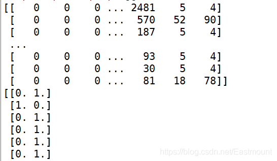
After obtaining the feature word number, that is, the header of the feature matrix is defined. Next, we need to convert each line of text into a one-dimensional word vector, and finally construct the feature matrix for training and classification. Note that using pad_sequences method unifies the length of CNN training to better train. For example, if the sentence is set to 100, the words behind it will be cut off if the sentence exceeds 100; If the sentence does not exceed 100, 0 will be filled in front of the sentence. The following figure shows the process of filling 0. At the same time, the classification result [0,1] indicates that the class mark is a positive 0, [1,0] indicates that the class mark is a negative 1.
The complete code at this time is as follows:
# Using train_test_split split X y list
X_train, X_test, y_train, y_test = train_test_split(Mat, labels, test_size=0.3, random_state=1)
print(X_train[:5])
print(y_train[:5])

#----------------------------------Step 3: word vector construction--------------------------------
# Word2Vec training
maxLen = 100                 #Maximum length of word sequence
num_features = 100           #Set word vector dimension
min_word_count = 3           #Ensure the minimum frequency of words considered
num_workers = 4              #Set parallel training and use CPU to calculate the number of cores
context = 4                  #Set word context window size

# Set model
model = word2vec.Word2Vec(Mat, workers=num_workers, size=num_features,
                          min_count=min_word_count,window=context)
# Forced unit normalization
model.init_sims(replace=True)
# Enter a path to save the training model/ The data/model directory exists beforehand
model.save("CNNw2vModel")
model.wv.save_word2vec_format("CNNVector",binary=False)
print(model)
# Load the model. If word2vec has been trained, use the following statement directly
w2v_model = word2vec.Word2Vec.load("CNNw2vModel")

# Feature number (fill 0 in front of insufficient)
trainID = tokenizer.texts_to_sequences(X_train)
print(trainID)
testID = tokenizer.texts_to_sequences(X_test)
print(testID)
# This method will unify the length of CNN training
trainSeq = pad_sequences(trainID, maxlen=maxLen)
print(trainSeq)

# Label independent hot coding is converted to one hot coding
trainCate = to_categorical(y_train, num_classes=2) #Second classification problem
print(trainCate)
testCate = to_categorical(y_test, num_classes=2)  #Second classification problem
print(testCate)
The output results are as follows:
[['scenery', ' ', 'scenic spot', 'too', 'mature', 'from', 'large', 'waterfall', 'scenic spot', 'set out', 'scenic spot', 'Sightseeing car', 'Sufficient', 'tourist', 'Semih.', 'the World Expo', 'On the way', 'jostle one another on the way', 'appreciate', 'beautiful scenery', 'mood', 'Sightseeing car', 'Get in the car', 'place', 'Indicate', 'destination', 'entrance', 'guide', 'go', 'Wronged Road', 'Muddle headed', 'Get in the car', 'ask', 'driver', 'arrive', 'driver', 'Vaguely', 'say', 'Out', 'scenic spot', 'passenger station', 'Seven holes', 'scenic spot', 'development', 'perfect', 'Put away', 'comment'],
['Low Season', 'waterfall', 'people', 'less', 'Jingmei', 'plane ticket', 'cheap', 'worth', 'go'],
['waterfall', 'experience', 'difference', 'Five stars', 'Praise', 'whole', 'yes', 'brush', 'road', 'Very narrow', 'cause', 'large area', 'blocking', 'line up', 'collapse', 'scenic spot', 'guide', 'clear', 'line up', 'heavy rain', 'Shelter from rain', 'Design', 'get', 'adult', 'child', 'the elderly', 'get wet in the rain', 'scenic spot', 'Reception', 'Poor ability', 'waterfall', 'really', 'enjoy undeserved fame', 'Seven holes', 'Put away', 'comment'],
['daddy', 'branch', 'waterfall', 'waterfall', 'waterfall', 'visit', 'waterfall', 'admission ticket', 'anyway', 'exceed', ' ', 'come', 'be familiar with', 'inform', 'can only', 'Out', 'get into', 'mouth', 'go back to', 'high speed', 'Export', 'Straight ahead', 'go back', 'inverted', 'instructions', 'clear', 'quarantine', 'Railing', 'Self driving', 'Lead in', 'Parking lot', 'Parking lot', 'charge', 'And', 'time', ' ', 'Parking lot', 'After investigation', 'scenic spot', 'admission ticket', 'Single', 'contain', 'traffic', 'fare', 'Traffic vehicle', 'need', 'Extra payment', 'From outside', 'around', 'road', 'flower', 'Less than', 'minute', 'fare', 'sincerely', 'accept', ' ', 'whole family', 'No', '┐', '(', '─', '__', '─', ')', '┌', 'interest', 'Collusion', 'severe', 'Fee increase', 'Gejin', 'waterfall', 'good-looking', 'difference', 'review', ' ', 'picture', 'not', 'development', 'waterfall', 'Tiankeng', 'waterfall', 'Spectacular', 'Spectacular', 'have', 'Smart', 'scenic spot', 'expand', 'become', 'Put away', 'comment'],
['whole family', 'ticket', 'resident', 'vip ', 'Discount', 'ticket']]

[1, 0, 1, 1, 1]
Word2Vec(vocab=718, size=100, alpha=0.025)

[[   0    0    0 ... 2481    5    4]
 [   0    0    0 ...  570   52   90]
 [   0    0    0 ...  187    5    4]
 ...
 [   0    0    0 ...   93    5    4]
 [   0    0    0 ...   30    5    4]
 [   0    0    0 ...   81   18   78]]

 [[0. 1.]
 [1. 0.]
 [0. 1.]
 [0. 1.]
 [0. 1.]
 [0. 1.]
 [1. 0.]
3.CNN construction
Next, we begin to train the constructed feature matrix and calculate the similarity of different texts or one-dimensional matrix. In this way, different sentences with good and bad comments will be divided into two categories according to the similarity. Word2Vec is also used here. The core code is as follows:
model = word2vec.Word2Vec(
	Mat,
	workers=num_workers,
	size=num_features,
	min_count=min_word_count,
	window=context
);
The result of the training model is "Word2Vec(vocab=718, size=100, alpha=0.025)". The filtering frequency set here is 3, which is equivalent to filtering those whose frequency is lower than 3, and finally 718 feature words are obtained. num_ The features value is 100, indicating that it is a 100 dimensional word vector. sg defaults to continuous word bag model, and can also be set to 1-hop word model. The default optimization method is negative sampling. Please read Baidu for more parameter explanations.
Refer to the author's previous article: [Python artificial intelligence] IX gensim word vector Word2Vec installation and similarity meter of Chinese short text of Qingnian
If we have a training set and a test set, how can we solve it if there is no feature word in the test set? Here, we use try except exception capture when obtaining the word vector of a feature word and converting it into a training matrix. If the feature word is not found, we can skip it and it will automatically fill in 0.
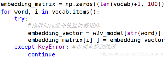
The code of this part is as follows:
#----------------------------------Step 4 CNN construction--------------------------------
# Use Word2vec after training to customize the training matrix of Embedding. Each line represents a word (combined with unique heat coding and matrix multiplication)
embedding_matrix = np.zeros((len(vocab)+1, 100)) #Counting from 0 plus 1 corresponds to the previous feature word
for word, i in vocab.items():
try:
#Extract the word vector and place the training matrix
embedding_vector = w2v_model[str(word)]
embedding_matrix[i] = embedding_vector
except KeyError: #Word not found skip
continue
# Training model
main_input = Input(shape=(maxLen,), dtype='float64')
# Word embedding uses the word vector of pre trained Word2Vec. The custom weight matrix 100 is the output word vector dimension
embedder = Embedding(len(vocab)+1, 100, input_length=maxLen,
weights=[embedding_matrix], trainable=False) #No more training
# Model building
model = Sequential()
model.add(embedder) #Building the Embedding layer
model.add(Conv1D(256, 3, padding='same', activation='relu')) #Convolution layer stride 3
model.add(MaxPool1D(maxLen-5, 3, padding='same')) #Pool layer
model.add(Conv1D(32, 3, padding='same', activation='relu')) #Convolution layer
model.add(Flatten()) #Straightening
model.add(Dropout(0.3)) #Prevent over fitting and 30% non training
model.add(Dense(256, activation='relu')) #Full connection layer
model.add(Dropout(0.2)) #Prevent overfitting
model.add(Dense(units=2, activation='softmax')) #Output layer
# Model visualization
model.summary()
# Activating neural network
model.compile(optimizer = 'adam', #optimizer
loss = 'categorical_crossentropy', #loss
metrics = ['accuracy'] #Calculation error or accuracy
)
#Training (training data, training category standard, batch size, 256 training each time, epochs, random selection, verification set 20%)
history = model.fit(trainSeq, trainCate, batch_size=256,
epochs=6, validation_split=0.2)
model.save("TextCNN")
#----------------------------------Step 5 prediction model--------------------------------
# Prediction and evaluation
mainModel = load_model("TextCNN")
result = mainModel.predict(testSeq) #Test sample
#print(result)
print(np.argmax(result,axis=1))
score = mainModel.evaluate(testSeq,
testCate,
batch_size=32)
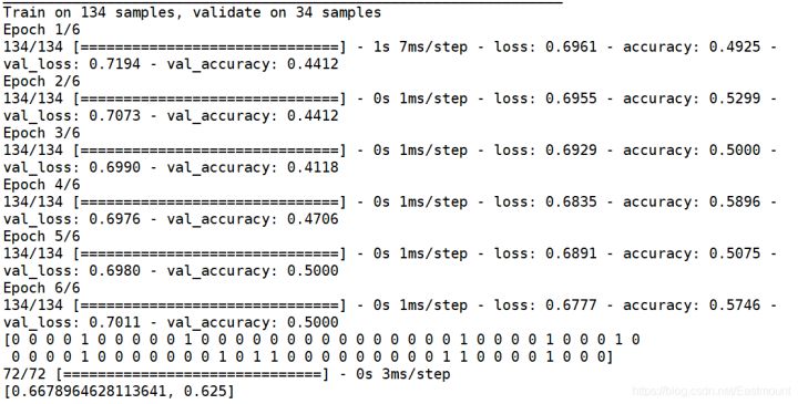
print(score)The constructed model is as follows:
Model: "sequential_1"
_________________________________________________________________
Layer (type)                 Output Shape              Param #
=================================================================
embedding_2 (Embedding)      (None, 100, 100)          290400
_________________________________________________________________
conv1d_1 (Conv1D)            (None, 100, 256)          77056
_________________________________________________________________
max_pooling1d_1 (MaxPooling1 (None, 34, 256)           0
_________________________________________________________________
conv1d_2 (Conv1D)            (None, 34, 32)            24608
_________________________________________________________________
flatten_1 (Flatten)          (None, 1088)              0
_________________________________________________________________
dropout_1 (Dropout)          (None, 1088)              0
_________________________________________________________________
dense_1 (Dense)              (None, 256)               278784
_________________________________________________________________
dropout_2 (Dropout)          (None, 256)               0
_________________________________________________________________
dense_2 (Dense)              (None, 2)                 514
=================================================================
Total params: 671,362
Trainable params: 380,962
Non-trainable params: 290,400
The output result is shown in the figure below. The prediction result of the model is not very ideal, and the accuracy value is only 0.625. Why? The author is also further studying the optimization of depth model. What is more important in this paper is to provide an available method. Please forgive me if the effect is not good~
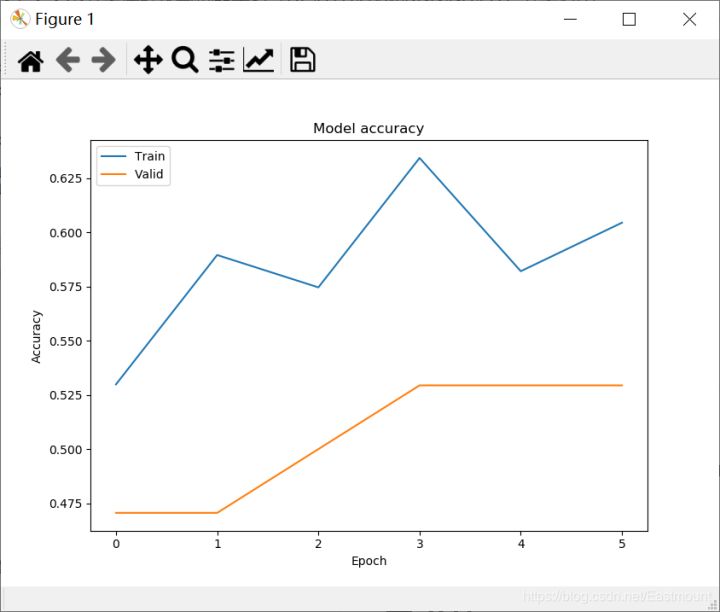
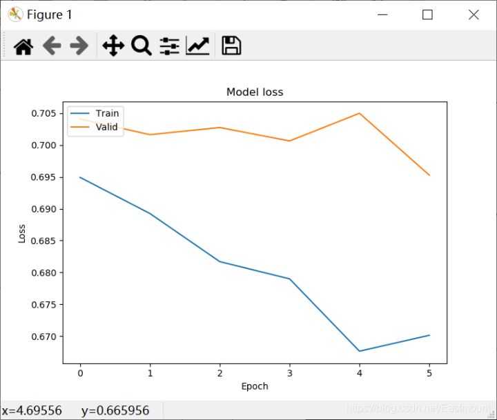
4. Test visualization
Finally, add visual code and draw graphics as shown in the figure below. Again, the effect of the algorithm is really not ideal, the error is not gradually decreasing, and the accuracy is not increasing. If readers find the reason or optimization method, please let us know. Thank you.
Finally, attach the complete code:
# -*- coding:utf-8 -*-
import csv
import numpy as np
import jieba
import jieba.analyse
import jieba.posseg as pseg
from sklearn import feature_extraction
from sklearn.feature_extraction.text import TfidfVectorizer
from sklearn.feature_extraction.text import CountVectorizer
from sklearn.feature_extraction.text import TfidfTransformer
from sklearn.model_selection import train_test_split
from sklearn.metrics import classification_report
from keras import models
from keras import layers
from keras import Input
from gensim.models import word2vec
from keras.preprocessing.text import Tokenizer
from keras.utils.np_utils import to_categorical
from keras.preprocessing.sequence import pad_sequences
from keras.models import Model
from keras.models import Sequential
from keras.models import load_model
from keras.layers import Flatten, Dense, Dropout, Conv1D, MaxPool1D, Embedding

#----------------------------------Step 1 data preprocessing--------------------------------
file = "data.csv"

# Get stop words
def stopwordslist(): #Load stop list
    stopwords = [line.strip() for line in open('stop_words.txt', encoding="UTF-8").readlines()]
    return stopwords

# Remove stop words
def deleteStop(sentence):
    stopwords = stopwordslist()
    outstr = ""
    for i in sentence:
        # print(i)
        if i not in stopwords and i!="\n":
            outstr += i
    return outstr

# Chinese word segmentation
Mat = []
with open(file, "r", encoding="UTF-8") as f:
    # Using CSV Dictreader reads the information in the file
    reader = csv.DictReader(f)
    labels = []
    contents = []
    for row in reader:
        # Data element acquisition
        if row['label'] == 'Praise':
            res = 0
        else:
            res = 1
        labels.append(res)

        # Chinese word segmentation
        content = row['content']
        #print(content)
        seglist = jieba.cut(content,cut_all=False)  #Precise mode
        #print(seglist)

        # De stop word
        stc = deleteStop(seglist) #Note that there are no spaces in the sentence
        # Space splicing
        seg_list = jieba.cut(stc,cut_all=False)
        output = ' '.join(list(seg_list))
        #print(output)
        contents.append(output)

        # Part of speech tagging
        res = pseg.cut(stc)
        seten = []
        for word,flag in res:
            if flag not in ['nr','ns','nt','mz','m','f','ul','l','r','t']:
                #print(word,flag)
                seten.append(word)
        Mat.append(seten)

print(labels[:5])
print(contents[:5])
print(Mat[:5])

#----------------------------------Step 2 feature number--------------------------------
# fit_ on_ The texts function can number each word of the input text according to the word frequency (the greater the word frequency, the smaller the number)
tokenizer = Tokenizer()
tokenizer.fit_on_texts(Mat)
vocab = tokenizer.word_index  #Stop words have been filtered. Get the number of each word
print(vocab)

# Using train_test_split split X y list
X_train, X_test, y_train, y_test = train_test_split(Mat, labels, test_size=0.3, random_state=1)
print(X_train[:5])
print(y_train[:5])

#----------------------------------Step 3: word vector construction--------------------------------
# Word2Vec training
maxLen = 100                 #Maximum length of word sequence
num_features = 100           #Set word vector dimension
min_word_count = 3           #Ensure the minimum frequency of words considered
num_workers = 4              #Set parallel training and use CPU to calculate the number of cores
context = 4                  #Set word context window size

# Set model
model = word2vec.Word2Vec(Mat, workers=num_workers, size=num_features,
                          min_count=min_word_count,window=context)
# Forced unit normalization
model.init_sims(replace=True)
# Enter a path to save the training model/ The data/model directory exists beforehand
model.save("CNNw2vModel")
model.wv.save_word2vec_format("CNNVector",binary=False)
print(model)
# Load the model. If word2vec has been trained, use the following statement directly
w2v_model = word2vec.Word2Vec.load("CNNw2vModel")

# Feature number (fill 0 in front of insufficient)
trainID = tokenizer.texts_to_sequences(X_train)
print(trainID)
testID = tokenizer.texts_to_sequences(X_test)
print(testID)
# This method will unify the length of CNN training
trainSeq = pad_sequences(trainID, maxlen=maxLen)
print(trainSeq)
testSeq = pad_sequences(testID, maxlen=maxLen)
print(testSeq)

# Label independent hot coding is converted to one hot coding
trainCate = to_categorical(y_train, num_classes=2) #Second classification problem
print(trainCate)
testCate = to_categorical(y_test, num_classes=2)  #Second classification problem
print(testCate)

#----------------------------------Step 4 CNN construction--------------------------------
# Use Word2vec after training to customize the training matrix of Embedding. Each line represents a word (combined with unique heat coding and matrix multiplication)
embedding_matrix = np.zeros((len(vocab)+1, 100)) #Counting from 0 plus 1 corresponds to the previous feature word
for word, i in vocab.items():
    try:
        #Extract the word vector and place the training matrix
        embedding_vector = w2v_model[str(word)]
        embedding_matrix[i] = embedding_vector
    except KeyError: #Word not found skip
        continue

# Training model
main_input = Input(shape=(maxLen,), dtype='float64')
# Word embedding uses the word vector of pre trained Word2Vec. The custom weight matrix 100 is the output word vector dimension
embedder = Embedding(len(vocab)+1, 100, input_length=maxLen,
                     weights=[embedding_matrix], trainable=False) #No more training
# Model building
model = Sequential()
model.add(embedder)  #Building the Embedding layer
model.add(Conv1D(256, 3, padding='same', activation='relu')) #Convolution layer stride 3
model.add(MaxPool1D(maxLen-5, 3, padding='same'))            #Pool layer
model.add(Conv1D(32, 3, padding='same', activation='relu'))  #Convolution layer
model.add(Flatten())                                         #Straightening
model.add(Dropout(0.3))                                      #Prevent over fitting and 30% non training
model.add(Dense(256, activation='relu'))                     #Full connection layer
model.add(Dropout(0.2))                                      #Prevent overfitting
model.add(Dense(units=2, activation='softmax'))              #Output layer

# Model visualization
model.summary()

# Activating neural network
model.compile(optimizer = 'adam',                    #optimizer
              loss = 'categorical_crossentropy',     #loss
              metrics = ['accuracy']                 #Calculation error or accuracy
              )

#Training (training data, training category standard, batch size, 256 training each time, epochs, random selection, verification set 20%)
history = model.fit(trainSeq, trainCate, batch_size=256,
                    epochs=6, validation_split=0.2)
model.save("TextCNN")

#----------------------------------Step 5 prediction model--------------------------------
# Prediction and evaluation
mainModel = load_model("TextCNN")
result = mainModel.predict(testSeq) #Test sample
print(result)
print(np.argmax(result,axis=1))
score = mainModel.evaluate(testSeq,
                           testCate,
                           batch_size=32)
print(score)

#----------------------------------Step 5 visualization--------------------------------
import matplotlib.pyplot as plt
plt.plot(history.history['accuracy'])
plt.plot(history.history['val_accuracy'])
plt.title('Model accuracy')
plt.ylabel('Accuracy')
plt.xlabel('Epoch')
plt.legend(['Train','Valid'], loc='upper left')

plt.plot(history.history['loss'])
plt.plot(history.history['val_loss'])
plt.title('Model loss')
plt.ylabel('Loss')
plt.xlabel('Epoch')
plt.legend(['Train','Valid'], loc='upper left')
plt.show()
IV summary
In short, this paper implements a case of CNN text classification learning through Keras, and introduces the principle knowledge of text classification and its comparison with machine learning in detail.
Click follow to learn about Huawei's new cloud technology for the first time~