1. Overview

1.1 What is Factor Analysis

Factor analysis originated from the fact that in 1904 a British psychologist found a strong correlation between students'English, French and classical performance, believing that there was a common driver behind the three courses and defining it as "language competence". Based on this idea, we find that many highly correlated factors are driven by a common factor, thus defining factor analysis.

Factor analysis is often used in the fields of economics, psychology, linguistics and sociology, and generally explores the underlying factors such as language ability, intelligence, comprehension, etc. These are common factors that cannot be calculated directly but are based on the research data behind them.

In summary, factor analysis is to extract variables with some correlation into fewer factors, use these factors to represent the original variables, or classify them according to the factors.

1.2 What to Solve

1. In multivariate scenarios, mining the impact factors behind

2. Dimension reduction before mathematical modeling

2. Steps

Factor analysis is to find a linear combination of nonlinearly related "variables" to represent the original variables, which are called factors. In the following figure, F is the factor, X is the original variable, and eps is the part of the original variable that cannot be represented by a common factor.

 

 

 

 

The above formulas need to be satisfied:

1. Requires that the data for the factor be less than the number of original variables, that is, m < p;
2. Factor F is independent of each other and has a variance of 1.
3. The correlation between factor F and eps is 0, and that between eps is 0.

Therefore, the process of factor analysis is to achieve the following objectives:

1. The coefficients of the factor F in the solution equation;
2. Give the actual explanation of factor F;
3. Show the relationship between the original features and public factors to achieve the purposes of dimension reduction and feature classification.

1) Sufficiency Test

• Objective: To test whether there is a correlation between variables to determine whether it is suitable for factor analysis.
• Methods: Sampling suitability test (KMO test) or Bartlett's Test.

 

 

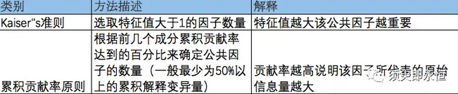
2) Number of selection factors

• Objective: To define the most appropriate number of potential public factors through data, and to determine the effect of factor analysis after that.
• Method: Kaiser's criterion or the principle of cumulative contribution rate.

 

 

3) Extracting common factors and rotating them

Extracting the common factor is the process of solving the function mentioned above. The general solutions are: principal component method, maximum likelihood method, minimum residual method and so on.

The reason for the factor rotation is that there are many solutions for extracting the common factor, and the factor load matrix is redistributed after the factor rotation, making it easier to interpret the rotated factor. The most common method is the maximum variance method.

4) Explain and name factors

• Purpose: Interpretation and naming are actually the process of understanding potential factors; This step is critical and requires a good understanding of the business. This is also the main reason why we use factor analysis.
• Methods: According to the characteristics of factor load matrix, the factor was found.

5) Calculating factor score

For each sample, their specific data values on different factors are obtained, which are the factor scores.

Step 1: Data preprocessing and analysis

###Standardization
scaler = StandardScaler().fit(data_9) #Declare the class and use fit()Method Computing Subsequent Standardized mean and std
print('\n Mean:',scaler.mean_)    #Class properties: mean
print('Variance:',scaler.var_)     #Class properties: variance

x_scaler = scaler.transform(data_9)  #Transformation X
print('\n Standardized data:\n',x_scaler)

Step 2: Factor Analysis - Sufficiency Test

Bartlett P value is less than 0.01 and KMO value is greater than 0.6; This data is suitable for factor analysis.

## Adequacy testing
### p value less than 0.01, kmo value greater than 0.6
from factor_analyzer.factor_analyzer import calculate_bartlett_sphericity
from factor_analyzer.factor_analyzer import calculate_kmo

chi_val,p_val = calculate_bartlett_sphericity(x_scaler)
kmo_all,kmo_val = calculate_kmo(x_scaler)
print(p_val,kmo_val)

Step 3: Determine the number of factors

There are two factors with eigenvalues greater than 1, and the cumulative variance of the two factors is 68%; Therefore, the number of factors is determined to be 2.

###Number of factors determination
from factor_analyzer import FactorAnalyzer

fa = FactorAnalyzer(x_scaler.shape[1],rotation=None)
fa.fit(x_scaler)
eigen_val,eigen_vector = fa.get_eigenvalues()
var = fa.get_factor_variance
print(eigen_val)
print(eigen_vector)
print(var)

Step 4: Factor analysis

The factor analysis function is invoked and the factor load matrix is obtained.

### factor analysis
fa = FactorAnalyzer(2,rotation='varimax')
fa.fit(x_scaler)

df_loading = pd.DataFrame(fa.loadings_,index=header_name[7:16])
df_loading

Step 5: Calculate Factor Score

### Calculating factor score
data_trans = pd.DataFrame(fa.transform(x_scaler))
plt.scatter(data_trans.loc[:,0],data_trans.loc[:,1])
plt.title("Factor Score")
plt.xlabel("factor1")
plt.ylabel("factor2")
plt.grid()
plt.show()