Here, we will introduce and explain the feature data selection methods often used in Feature Engineering, which are divided into three parts: single variable selection, linear model selection and random forest model feature selection.
Trilogy 1: single variable selection
For data scientists or machine learning practitioners, a good understanding of feature selection / sequencing can be a valuable asset. A good grasp of these methods can lead to a better performance model, a better understanding of the underlying structure and characteristics of data, and a better understanding of the algorithms that form the basis of many machine learning models.
There are usually two reasons to use feature selection:
1. Reduce the number of features to reduce over fitting and improve the generalization of the model.
2. Better understand the function and its relationship with response variables.
These two goals often contradict each other, so different methods are needed: according to the data at hand, the feature selection method beneficial to goal (1) is not necessarily beneficial to goal (2), and vice versa. However, what seems to happen frequently is that people use their favorite methods (or the most convenient methods from the selected tools) indiscriminately, especially the methods that are more suitable for (1) implementation (2).
At the same time, machine learning or data mining textbooks do not introduce function selection in detail, in part because they are usually regarded as the natural side effects of learning algorithms and do not need to be introduced separately.
In this blog post, I will try to introduce some of the more popular function selection methods and their advantages and disadvantages, as well as code examples in Python and scikit learn. I will also run these methods side-by-side in the sample dataset, which highlights some of the major differences between them. In all of the examples, I'm focused on regression datasets, but most of the discussions and examples apply equally to classification datasets and methods.
Single variable feature selection
Single variable feature selection checks each feature individually to determine the strength of the relationship between the feature and the response variable. These methods are easy to run and understand, and are often particularly useful for better understanding of data (but do not necessarily optimize feature sets for better versatility). There are many different options for single variable selection.
Pearson correlation
One of the simplest ways to understand the relationship between elements and response variables is Pearson correlation coefficient, which can measure the linear correlation between two variables. The result value is at [- 1; 1], where - 1 is the total negative correlation (the other variable decreases as one variable increases), + 1 is the total positive correlation, and 0 is the no linear correlation between the two variables.
It's fast and easy to calculate, and it's usually the first thing to do with data. Scipy's pearsonr method calculates correlation and correlation's p value at the same time, which roughly shows the possibility of uncorrelated system to create this size correlation value.
import numpy as np
from scipy.stats import pearsonr
np.random.seed(0)
size = 300
x = np.random.normal(0, 1, size)
print "Lower noise", pearsonr(x, x + np.random.normal(0, 1, size))
print "Higher noise", pearsonr(x, x + np.random.normal(0, 10, size))
The results are as follows:
Lower noise (0.71824836862138386, 7.3240173129992273e-49)
Higher noise (0.057964292079338148, 0.31700993885324746)
As you can see from the example, we compare variables to their noisy versions. When the noise is small, the correlation is relatively strong, and the p value is very low. In the noisy comparison, the correlation is very small, and the p value is very high, which means that it is likely to observe that the correlation is completely accidental.
Scikit learn provides f_regrssion method is used to calculate the p value (and basic F value) of a group of elements in batch. Therefore, it is a convenient method to carry out an association test on the data set, such as including it in the pipeline of sklearn.
The obvious disadvantage of Pearson correlation as a feature ranking mechanism is that it is only sensitive to linear relationship. If the relationship is nonlinear, the Pearson correlation can be close to zero even if there is a 1-1 correspondence between the two variables.
For example, when x is centered on 0, the correlation between X and x2 is zero.
x = np.random.uniform(-1, 1, 100000)
print pearsonr(x, x**2)[0]
The results are as follows:
-0.00230804707612
For more examples similar to the above, see the following example diagram.
In addition, as Anscombe's Quartet shows, relying solely on correlation values to explain the relationship between the two variables can be extremely misleading, so it is always worth plotting the data.
Mutual information and maximum information coefficient (MIC)
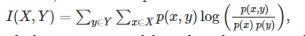
Another more reliable option for correlation estimation is mutual information, which is defined as:
It measures the interdependence of variables, usually in bits.
But for two reasons, it may not be convenient to use it directly in feature ranking. First of all, it is not an indicator, nor is it standardized (that is, it is not in a fixed range), so MI values are incomparable between two data sets. Secondly, the calculation of continuous variables may be inconvenient: usually, variables need to be discretized through sub boxes, but the mutual information score may be very sensitive to the selection of sub boxes.
The maximum information coefficient is a technology developed to solve these shortcomings. It searches for the best box and converts the mutual information score into a measure of the range [0; 1]. In python, MIC is available in the minepy library.
Looking back at the example of y = x2, MIC found that the mutual information is 1, which is the largest.
from minepy import MINE
m = MINE()
x = np.random.uniform(-1, 1, 10000)
m.compute_score(x, x**2)
print m.mic()
The results are as follows:
1.0
People have criticized the statistical ability of MIC, that is, when the original hypothesis is false, we can reject the original hypothesis. Depending on the particular data set and how noisy it is, this may or may not be a problem.
Distance correlation
Another powerful competitive method of correlation estimation is distance correlation, which is specially designed to solve the problem of Pearson correlation. Although for Pearson correlation, a correlation value of 0 does not indicate independence (as can be seen from the x vs x2 example), a distance correlation of 0 indicates that there is no correlation between the two variables.
Distance dependency is provided, for example, in R's energy pack (and Python's point).
#R-code
> x = runif (1000, -1, 1)
> dcor(x, x**2)
[1] 0.4943864
When the relationship is nearly linear, there are at least two reasons for favoring Pearson correlation over more complex methods such as MIC or distance correlation. On the one hand, calculating Pearson correlation is much faster, which may be important for large data sets. Second, the range of correlation coefficients is [- 1; 1] (not MIC and distance related [0; 1]). This can convey useful additional information about whether the relationship is negative or positive, i.e. whether a higher eigenvalue implies a higher value for the response variable, and vice versa. But, of course, only when the relationship between the two variables is monotonous, the problem of negative correlation and positive correlation is appropriate.
Model based ranking
Finally, any machine learning method can be used, and each individual function can be used to build a prediction model for the response variables, and measure the performance of each model. In fact, this has been used with Pearson's correlation coefficient because it is equivalent to the standardized regression coefficient used for linear regression prediction. If the relationship between features and response variables is nonlinear, there are many alternative methods, such as tree based method (decision tree, random forest), linear model with basic expansion, etc. Tree based methods may be one of the simplest to apply because they can model nonlinear relationships well and do not require much adjustment. The main thing to avoid is over fitting, so the depth of the tree should be relatively small and cross validation should be applied.
This is a single variable selection using sklearn's random forest regression on the Boston housing price data set. This sample contains housing prices and many key attributes in suburban Boston.
from sklearn.cross_validation import cross_val_score, ShuffleSplit
from sklearn.datasets import load_boston
from sklearn.ensemble import RandomForestRegressor

#Load boston housing dataset as an example
boston = load_boston()
X = boston["data"]
Y = boston["target"]
names = boston["feature_names"]

rf = RandomForestRegressor(n_estimators=20, max_depth=4)
scores = []
for i in range(X.shape[1]):
     score = cross_val_score(rf, X[:, i:i+1], Y, scoring="r2",
                              cv=ShuffleSplit(len(X), 3, .3))
     scores.append((round(np.mean(score), 3), names[i]))
print sorted(scores, reverse=True)
The results are as follows:
[(0.636, 'LSTAT'), (0.59, 'RM'), (0.472, 'NOX'), (0.369, 'INDUS'), (0.311, 'PTRATIO'), (0.24, 'TAX'), (0.24, 'CRIM'), (0.185, 'RAD'), (0.16, 'ZN'), (0.087, 'B'), (0.062, 'DIS'), (0.036, 'CHAS'), (0.027, 'AGE')]
Trilogy two: linear model and regularization
In my previous article, I discussed single variable feature selection, where each feature is evaluated independently of the response variable. Another popular method is to use machine learning model for feature ranking. Many machine learning models have some inherent internal feature levels, or they can easily generate levels from the structure of the model. It is suitable for regression model, SVM, decision tree, random forest and so on.
In this article, I will discuss the use of regression model coefficients to select and interpret features. This is based on the following idea: when all features are in the same scale, the most important feature should have the highest coefficient in the model, while the features that are not related to the output variables should have a coefficient value close to zero. When the data is not too noisy (or there is a lot of data compared with the number of elements) and the elements are (relatively) independent, the method can work well even if a simple linear regression model is used:
from sklearn.linear_model import LinearRegression
import numpy as np

np.random.seed(0)
size = 5000

#A dataset with 3 features
X = np.random.normal(0, 1, (size, 3))
#Y = X0 + 2*X1 + noise
Y = X[:,0] + 2*X[:,1] + np.random.normal(0, 2, size)
lr = LinearRegression()
lr.fit(X, Y)

#A helper method for pretty-printing linear models
def pretty_print_linear(coefs, names = None, sort = False):
    if names == None:
        names = ["X%s" % x for x in range(len(coefs))]
    lst = zip(coefs, names)
    if sort:
        lst = sorted(lst,  key = lambda x:-np.abs(x[0]))
    return " + ".join("%s * %s" % (round(coef, 3), name)
                                   for coef, name in lst)

print "Linear model:", pretty_print_linear(lr.coef_)
The results are as follows:
Linear model: 0.984 * X0 + 1.995 * X1 + -0.041 * X2
As you can see in this example, although there is a lot of noise in the data, the model does restore the data infrastructure well. But in fact, this learning problem is particularly suitable for linear models: the pure linear relationship between features and response variables, but there is no correlation between features.
When there are multiple (linear) correlation features (like many real-life data sets), the model becomes unstable, which means that small changes in the data will lead to large changes in the model (i.e. coefficient value), so it is very difficult to explain the model (so-called multicollinearity problem). For example, suppose we have a dataset where the "real" model of the data is Y = X1 + X2, and we observe Y ^ = X1 + X2 + ϵ, where ϵ is noise. In addition, it is assumed that X1 is linearly related to X2, so that x1 ≈ x2. Ideally, the learning model would be Y = X1 + X2. But according to the amount of noise ϵ, the amount of data at hand and the correlation between X1 and X2, it may also be Y = 2X1 (i.e. only X1 is used as the prediction variable) or Y = -X1 + 3X2 (the coefficient may be just suitable for noisy training set).
Let's look at the same related data set as the random forest example, with some noise added.
from sklearn.linear_model import LinearRegression

size = 100
np.random.seed(seed=5)

X_seed = np.random.normal(0, 1, size)
X1 = X_seed + np.random.normal(0, .1, size)
X2 = X_seed + np.random.normal(0, .1, size)
X3 = X_seed + np.random.normal(0, .1, size)

Y = X1 + X2 + X3 + np.random.normal(0,1, size)
X = np.array([X1, X2, X3]).T

lr = LinearRegression()
lr.fit(X,Y)
print "Linear model:", pretty_print_linear(lr.coef_)
The results are as follows:
Linear model: -1.291 * X0 + 1.591 * X1 + 2.747 * X2
The coefficients total about 3, so we can expect the learning model to perform well. On the other hand, if we want to explain the coefficients of face value, the model X3 has a strong positive impact on the output variables, while X1 has a negative impact. In fact, almost all functions are related to output variables.
The same methods and considerations apply to other similar linear methods, such as logistic regression.
Regularization model
Regularization is a method used to add other constraints or penalties to the model, in order to prevent over fitting and improve generalization. Instead of the minimum loss function E (X, Y), the minimum loss function becomes e (X, Y) + α ∥ w ∥ where W is the vector of the model coefficient, ∥ is usually L1 or L2 norm, α is the adjustable free parameter, and specifies the regularization amount (therefore α = 0 represents the non regularized model). For regression model, two widely used regularization methods are L1 and L2 regularization, which are also called lasso and ridge regression when applied in linear regression.
L1 regularization / Lasso
L1 regularization adds penalty α Σ ni = 1 | wi | to loss function (L1 norm). Since each non-zero coefficient increases the penalty, it forces the coefficient of the weak feature to be zero. Therefore, L1 regularization produces sparse solution, which inherently performs feature selection.
For regression, scikit learn provides Lasso for linear regression and Logistic regression, and L1 penalty score for classification.
Let's run lasso on a Boston housing dataset with good alpha values (for example, Lasso can be found by grid search):
from sklearn.linear_model import Lasso
from sklearn.preprocessing import StandardScaler
from sklearn.datasets import load_boston

boston = load_boston()
scaler = StandardScaler()
X = scaler.fit_transform(boston["data"])
Y = boston["target"]
names = boston["feature_names"]

lasso = Lasso(alpha=.3)
lasso.fit(X, Y)

print "Lasso model: ", pretty_print_linear(lasso.coef_, names, sort = True)
The results are as follows:
Lasso model: -3.707 * LSTAT + 2.992 * RM + -1.757 * PTRATIO + -1.081 * DIS + -0.7 * NOX + 0.631 * B + 0.54 * CHAS + -0.236 * CRIM + 0.081 * ZN + -0.0 * INDUS + -0.0 * AGE + 0.0 * RAD + -0.0 * TAX
We see that many features have a coefficient of 0. If α is further increased, the solution will be sparse and sparse, that is, more and more features have coefficients of 0.
Note, however, that the L1 regular regression is similar to the non regular linear model, so it is unstable, which means that even if there are relevant features in the data, even if there are small changes in the data, the coefficient (and feature level) may change significantly. This brings us to L2 regularization.
L2 regularization / Ridge regression
L2 regularization (called ridge regression of linear regression) adds L2 norm penalty (α Σ ni = 1w2i) to the loss function. Because the coefficient is square in the penalty expression, it has a different effect from L1 norm, that is, it forces the coefficient values to be more evenly distributed. For related features, this means that they tend to get similar coefficients. Back to the example of Y = X1 + X2, where X1 and X2 are highly correlated, for L1, the penalty is the same * x2 whether the learning model is Y = 1 * X1 + 1 * X2 or Y = 2 * X1 + 0. In both cases, the penalty is 2 * α. However, for L2, the penalty for the first model is 12 + 12 = 2 α, while for the second model, the penalty is 22 + 02 = 4 α.
As a result, the model is more stable (the coefficient does not fluctuate with small data changes, just like the irregular model or L1 model). Therefore, although L2 regularization performs different functional choices than L1, it is more useful for feature * interpretation *: prediction features will get non-zero coefficients, which L1 usually does not.
Let's look again at an example with three related characteristics, running the example 10 times with different random seeds to emphasize the stability of L2 regression.
from sklearn.linear_model import Ridge
from sklearn.metrics import r2_score
size = 100

#We run the method 10 times with different random seeds
for i in range(10):
    print "Random seed %s" % i
    np.random.seed(seed=i)
    X_seed = np.random.normal(0, 1, size)
    X1 = X_seed + np.random.normal(0, .1, size)
    X2 = X_seed + np.random.normal(0, .1, size)
    X3 = X_seed + np.random.normal(0, .1, size)
    Y = X1 + X2 + X3 + np.random.normal(0, 1, size)
    X = np.array([X1, X2, X3]).T


    lr = LinearRegression()
    lr.fit(X,Y)
    print "Linear model:", pretty_print_linear(lr.coef_)

    ridge = Ridge(alpha=10)
    ridge.fit(X,Y)
    print "Ridge model:", pretty_print_linear(ridge.coef_)
    print
The results are as follows:
Random seed 0
Linear model: 0.728 * X0 + 2.309 * X1 + -0.082 * X2
Ridge model: 0.938 * X0 + 1.059 * X1 + 0.877 * X2

Random seed 1
Linear model: 1.152 * X0 + 2.366 * X1 + -0.599 * X2
Ridge model: 0.984 * X0 + 1.068 * X1 + 0.759 * X2

Random seed 2
Linear model: 0.697 * X0 + 0.322 * X1 + 2.086 * X2
Ridge model: 0.972 * X0 + 0.943 * X1 + 1.085 * X2

Random seed 3
Linear model: 0.287 * X0 + 1.254 * X1 + 1.491 * X2
Ridge model: 0.919 * X0 + 1.005 * X1 + 1.033 * X2

Random seed 4
Linear model: 0.187 * X0 + 0.772 * X1 + 2.189 * X2
Ridge model: 0.964 * X0 + 0.982 * X1 + 1.098 * X2

Random seed 5
Linear model: -1.291 * X0 + 1.591 * X1 + 2.747 * X2
Ridge model: 0.758 * X0 + 1.011 * X1 + 1.139 * X2

Random seed 6
Linear model: 1.199 * X0 + -0.031 * X1 + 1.915 * X2
Ridge model: 1.016 * X0 + 0.89 * X1 + 1.091 * X2

Random seed 7
Linear model: 1.474 * X0 + 1.762 * X1 + -0.151 * X2
Ridge model: 1.018 * X0 + 1.039 * X1 + 0.901 * X2

Random seed 8
Linear model: 0.084 * X0 + 1.88 * X1 + 1.107 * X2
Ridge model: 0.907 * X0 + 1.071 * X1 + 1.008 * X2

Random seed 9
Linear model: 0.714 * X0 + 0.776 * X1 + 1.364 * X2
Ridge model: 0.896 * X0 + 0.903 * X1 + 0.98 * X2
As you can see from the example, the coefficients of linear regression vary greatly according to the data generated. However, for the L2 regularization model, the coefficients are very stable and closely reflect the way of data generation (all coefficients are close to 1).
Trilogy three: random forest model selection
Importance of random forest characteristics
Random forest has become one of the most popular machine learning methods because of its relatively high accuracy, robustness and ease of use. They also provide two simple feature selection methods: average impurity reduction and average accuracy reduction.
Average impurity reduction
Random forest consists of many decision trees. Each node in the decision tree is a condition of a single function, which aims to divide the data set into two, so that the similar response values eventually reside in the same set. The measure on which the best (local) conditions are selected is called impurity. For classification, it is usually Gini impurity or information gain / entropy, while for regression tree it is variance. Therefore, when training a tree, we can calculate how much each feature reduces the weighted impurities in a tree. For the forest, the impurity reduction of each feature can be averaged and the features can be ranked according to this metric.
This is a measure of the functional importance of sklearn's "random forest" implementation (random forest classifier and random forest regression).
from sklearn.datasets import load_boston
from sklearn.ensemble import RandomForestRegressor
import numpy as np
#Load boston housing dataset as an example
boston = load_boston()
X = boston["data"]
Y = boston["target"]
names = boston["feature_names"]
rf = RandomForestRegressor()
rf.fit(X, Y)
print "Features sorted by their score:"
print sorted(zip(map(lambda x: round(x, 4), rf.feature_importances_), names),
             reverse=True)
The results are as follows:
Features sorted by their score:
[(0.5298, 'LSTAT'), (0.4116, 'RM'), (0.0252, 'DIS'), (0.0172, 'CRIM'), (0.0065, 'NOX'), (0.0035, 'PTRATIO'), (0.0021, 'TAX'), (0.0017, 'AGE'), (0.0012, 'B'), (0.0008, 'INDUS'), (0.0004, 'RAD'), (0.0001, 'CHAS'), (0.0, 'ZN')]
When using impurity based ranking, some considerations need to be kept in mind. First, feature selection based on impurity reduction tends to select variables with more categories (see bias in the importance assessment of random forest variables). Secondly, when the data set has two (or more) correlation features, from the perspective of the model, any of these correlation features can be used as prediction variables, without a specific preference for other features. But once one of them is used, the other importance is greatly reduced, because the impurities that can be removed effectively have been removed by the first feature. As a result, they will become less important. This is not a problem when we want to use feature selection to reduce over fitting, because it makes sense to delete features that are mostly duplicated by other features. However, when interpreting the data, it may come to the wrong conclusion that one of the variables is a strong predictive variable, while the other variables in the same group are not important, but in fact they are very close to the response variables.
Because of the random selection of features at the time of each node creation, the impact of this phenomenon is reduced, but the effect is not completely eliminated. In the following example, we have three related variables X0, X1, X2, and there is no noise in the data, while the output variable is just the sum of these three characteristics:
size = 10000
np.random.seed(seed=10)
X_seed = np.random.normal(0, 1, size)
X0 = X_seed + np.random.normal(0, .1, size)
X1 = X_seed + np.random.normal(0, .1, size)
X2 = X_seed + np.random.normal(0, .1, size)
X = np.array([X0, X1, X2]).T
Y = X0 + X1 + X2

rf = RandomForestRegressor(n_estimators=20, max_features=2)
rf.fit(X, Y);
print "Scores for X0, X1, X2:", map(lambda x:round (x,3),
                                    rf.feature_importances_)
The results are as follows:
Scores for X0, X1, X2: [0.278, 0.66, 0.062]
When we calculate the importance of features, we find that X1 is more than 10 times more important than X2, while their "true" importance is very similar. Although there is no noise in the data, this still happens. We use 20 trees, random selection of features (only two of the three features are considered in each segmentation) and a data set large enough.
One thing to point out, however, is that the difficulty of explaining the importance / rank of related variables is not specific to random forests, but is applicable to most model-based feature selection methods.
Average reduction accuracy
Another popular feature selection method is to directly measure the influence of each feature on the accuracy of the model. The general idea is that replacing the value of each feature and measuring how much displacement will reduce the accuracy of the model. Obviously, for the unimportant variables, the arrangement should have little effect on the model accuracy, and the arrangement of the important variables should greatly reduce the model accuracy.
This method is not directly exposed in sklearn, but it is very simple to implement. Continue with the previous example of ranking elements in the Boston housing dataset:
from sklearn.cross_validation import ShuffleSplit
from sklearn.metrics import r2_score
from collections import defaultdict

X = boston["data"]
Y = boston["target"]

rf = RandomForestRegressor()
scores = defaultdict(list)

#crossvalidate the scores on a number of different random splits of the data
for train_idx, test_idx in ShuffleSplit(len(X), 100, .3):
    X_train, X_test = X[train_idx], X[test_idx]
    Y_train, Y_test = Y[train_idx], Y[test_idx]
    r = rf.fit(X_train, Y_train)
    acc = r2_score(Y_test, rf.predict(X_test))
    for i in range(X.shape[1]):
        X_t = X_test.copy()
        np.random.shuffle(X_t[:, i])
        shuff_acc = r2_score(Y_test, rf.predict(X_t))
        scores[names[i]].append((acc-shuff_acc)/acc)
print "Features sorted by their score:"
print sorted([(round(np.mean(score), 4), feat) for
              feat, score in scores.items()], reverse=True)
The results are as follows:
Features sorted by their score:
[(0.7276, 'LSTAT'), (0.5675, 'RM'), (0.0867, 'DIS'), (0.0407, 'NOX'), (0.0351, 'CRIM'), (0.0233, 'PTRATIO'), (0.0168, 'TAX'), (0.0122, 'AGE'), (0.005, 'B'), (0.0048, 'INDUS'), (0.0043, 'RAD'), (0.0004, 'ZN'), (0.0001, 'CHAS')]
In this example, LSTAT and RM are two functions that have a significant impact on model performance: replacing them reduces model performance by about 73% and 57%, respectively. Keep in mind that these measurements are only made after all of these functional training (and depending on these characteristics) has been performed on the model. This doesn't mean that if we train a model without these functions, the performance of the model will drop so much, because other relevant functions can be used instead.
Original address:
Feature selection – Part I: univariate selection
Selecting good features – Part II: linear models and regularization
Selecting good features – Part III: random forests
Some formulas in the article show problems. If you need to know more about them, it is suggested to read the original text.