1. Foreword

In a previous blog Code implementation of federal learning basic algorithm FedAvg Using numpy hand built neural network to realize FedAvg, the effect of hand built neural network has been very excellent, not

II. Data introduction

There are multiple clients in federated learning. Each client has its own data set, which they are unwilling to share.

The data set selected in this paper is the real power load data of ten districts / counties in a city in northern China from 2016 to 2019. The collection time interval is 1 hour, that is, there are 24 load values every day.

We assume that the power departments in these 10 regions are unwilling to share their own data, but they want to get a global model trained by all data.

In addition to the power load data, there is another alternative data set: the wind power data set. The two data sets are specified by the parameter type: type == 'load' indicates load data and 'wind' indicates wind power data.

Characteristic structure

The load value at the first 24 hours of a certain time and the relevant meteorological data at that time (such as temperature, humidity, pressure, etc.) are used to predict the load value at that time.

For the wind power data, the wind power values of the first 24 times of a certain time and the relevant meteorological data at that time are also used to predict the wind power value at that time.

Each region should reach an agreement on how to formulate the feature set. The characteristics of the data in each region used in this paper are consistent and can be used directly.

3. Federal learning

1. Overall framework

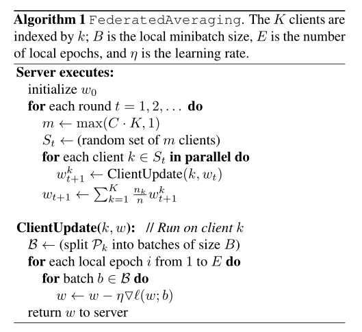
The framework of FedAvg proposed in the original paper is:

The client model is built by PyTorch:

class ANN(nn.Module):
    def __init__(self, input_dim, name, B, E, type, lr):
        super(ANN, self).__init__()
        self.name = name
        self.B = B
        self.E = E
        self.len = 0
        self.type = type
        self.lr = lr
        self.loss = 0
        self.fc1 = nn.Linear(input_dim, 20)
        self.relu = nn.ReLU()
        self.sigmoid = nn.Sigmoid()
        self.dropout = nn.Dropout()
        self.fc2 = nn.Linear(20, 20)
        self.fc3 = nn.Linear(20, 20)
        self.fc4 = nn.Linear(20, 1)

    def forward(self, data):
        x = self.fc1(data)
        x = self.sigmoid(x)
        x = self.fc2(x)
        x = self.sigmoid(x)
        x = self.fc3(x)
        x = self.sigmoid(x)
        x = self.fc4(x)
        x = self.sigmoid(x)

        return x

2. Server side

The server side performs the following steps:

1. Initialization parameters
2. For round t training: first calculate m = m a x ( C ⋅ K , 1 ) m=max(C \cdot K, 1) m=max(C ⋅ K,1), then randomly select m clients, and do the following operations for these m clients (all clients execute in parallel): update the local w t k w_t^{k} wtk # get w t + 1 k w_{t+1}^{k} wt+1k​. After all client updates are completed, the w t + 1 k w_{t+1}^{k} wt+1k is transmitted to the server, and the server integrates all w t + 1 k w_{t+1}^{k} wt+1k ， get the latest global parameters w t + 1 w_{t+1} wt+1​.
3. The server will the latest w t + 1 w_{t+1} wt+1 # distribute to all clients, and then carry out the next round of updates.

Simply put, in each round of communication, only some clients are selected. These clients use the local data to update the parameters, and then send them to the server. The server summarizes the parameters of all clients to form its own parameters, and then distributes the summarized parameters to all clients again, and then carry out the next round of update.

3. Client

The client has nothing to say, that is to update the parameters of the neural network model using local data.

4. Code implementation

4.1 initialization

Parameters:

1. K. The number of clients in this paper is 10, that is, 10 regions.
2. C: Selection rate: only C * K clients are selected in each round of communication.
3. E: When the client updates the parameters of the local model, it trains the e-round on the local data set.
4. B: When the client updates the parameters of the local model, the batch size of the local dataset is B
5. r: The server side and the client side conduct R rounds of communication.
6. Clients: collection of clients.
7. Type: Specifies the data type, load forecasting or wind power forecasting.
8. lr: learning rate.
9. input_dim: data input dimension.
10. nn: global model.
11. nns: client model collection.

Code implementation:

class FedAvg:
    def __init__(self, options):
        self.C = options['C']
        self.E = options['E']
        self.B = options['B']
        self.K = options['K']
        self.r = options['r']
        self.input_dim = options['input_dim']
        self.type = options['type']
        self.lr = options['lr']
        self.clients = options['clients']
        self.nn = ANN(input_dim=self.input_dim, name='server', B=B, E=E, type=self.type, lr=self.lr).to(device)
        self.nns = []
        for i in range(K):
            temp = copy.deepcopy(self.nn)
            temp.name = self.clients[i]
            self.nns.append(temp)

4.2 server side

The server code is as follows:

def server(self):
     for t in range(self.r):
          print('The first', t + 1, 'Round communication:')
          m = np.max([int(self.C * self.K), 1])
          # sampling
          index = random.sample(range(0, self.K), m)
          # local updating
          self.client_update(index)
          # aggregation
          self.aggregation()
          # dispatch
          self.dispatch()

     # return global model
     return self.nn

Where client_update(index):

def client_update(self, index):  # update nn
     for k in index:
          self.nns[k] = train(self.nns[k])

aggregation():

def aggregation(self):
     s = 0
     for j in range(self.K):
          # normal
          s += self.nns[j].len
          
     params = {}
     with torch.no_grad():
          for k, v in self.nns[0].named_parameters():
               params[k] = copy.deepcopy(v)
               params[k].zero_()
     for j in range(self.K):
          with torch.no_grad():
               for k, v in self.nns[j].named_parameters():
                    params[k] += v * (self.nns[j].len / s)
     with torch.no_grad():
          for k, v in self.nn.named_parameters():
               v.copy_(params[k])

dispatch():

def dispatch(self):
     params = {}
     with torch.no_grad():
          for k, v in self.nn.named_parameters():
               params[k] = copy.deepcopy(v)
     for j in range(self.K):
          with torch.no_grad():
               for k, v in self.nns[j].named_parameters():
                    v.copy_(params[k])

The following is an analysis of important codes:

• Client selection

m = np.max([int(self.C * self.K), 1])
index = random.sample(range(0, self.K), m)

The 0 ~ m integers in the selected index represent the 10 stored integers in the client.

• Client updates

for k in index:
    self.client_update(self.nns[k])

• The server side summarizes the parameters of the client model
  w t + 1 ← ∑ k = 1 K n k n w t + 1 k w_{t+1} \gets \sum_{k=1}^{K}\frac{n_k}{n}w_{t+1}^{k} wt+1​←k=1∑K​nnk​​wt+1k​
  among n k n_k nk ， indicates the second k k Local data volume of k clients. In other words, the more local data a client has, the greater the impact of its model on the global model.

Of course, this is only a very simple summary method, and there are other types of summary methods. paper Electricity Consumer Characteristics Identification: A Federated Learning Approach Three summary methods are summarized in:

1. normal: the method in the original paper, that is to determine the proportion of client parameters in the final combination according to the number of samples.
2. LA: the proportion of parameters in the final combination is determined according to the proportion of the loss of the client model in the sum of all client losses.
3. LS: determined according to the proportion of the product of the loss and the number of samples.

It is worth noting that although the server only selects m of the K clients to update each time, all client model parameters are finally summarized.

• Distribute the updated parameters to the client

def dispatch(self):
     params = {}
     with torch.no_grad():
          for k, v in self.nn.named_parameters():
               params[k] = copy.deepcopy(v)
     for j in range(self.K):
          with torch.no_grad():
               for k, v in self.nns[j].named_parameters():
                    v.copy_(params[k])

4.3 client

The client only needs to update with local data:

def client_update(self, index):  # update nn
     for k in index:
          self.nns[k] = train(self.nns[k])

train():

def train(ann):
    ann.train()
    # print(p)
    if ann.type == 'load':
        Dtr, Dte = nn_seq(ann.name, ann.B, ann.type)
    else:
        Dtr, Dte = nn_seq_wind(ann.named, ann.B, ann.type)
    ann.len = len(Dtr)
    # print(len(Dtr))
    loss_function = nn.MSELoss().to(device)
    loss = 0
    optimizer = torch.optim.Adam(ann.parameters(), lr=ann.lr)
    for epoch in range(ann.E):
        cnt = 0
        for (seq, label) in Dtr:
            cnt += 1
            seq = seq.to(device)
            label = label.to(device)
            y_pred = ann(seq)
            loss = loss_function(y_pred, label)
            # add mu/2*|w-wt|**2
            # temp = list(model.parameters())
            # loss += (mu / 2 * () ** 2)
            optimizer.zero_grad()
            loss.backward()
            optimizer.step()

        print('epoch', epoch, ':', loss.item())

    return ann

4.4 testing

def global_test(self):
     model = self.nn
     model.eval()
     c = clients if self.type == 'load' else clients_wind
     for client in c:
          model.name = client
          test(model)

4. Experiment and results

The parameters of this experiment are:

K	C	E	B	r
10	0.5	50	50	5

if __name__ == '__main__':
    K, C, E, B, r = 10, 0.5, 50, 50, 5
    type = 'load'
    input_dim = 30 if type == 'load' else 28
    _client = clients if type == 'load' else clients_wind
    lr = 0.08
    options = {'K': K, 'C': C, 'E': E, 'B': B, 'r': r, 'type': type, 'clients': _client,
               'input_dim': input_dim, 'lr': lr}
    fedavg = FedAvg(options)
    fedavg.server()
    fedavg.global_test()

The performance of each client on the local test set after individual training (50 rounds of training, batch size of 50) is as follows:

Client number	1	2	3	4	5	6	7	8	9	10
MAPE / %	5.33	4.11	3.03	4.20	3.02	2.70	2.94	2.99	2.30	4.10

It can be seen that because the data of each client is very sufficient, the prediction accuracy of the local model trained by each client has been very high.

After five rounds of communication between the server and the client, the performance of the global model on the server on the 10 client test sets is as follows:

Client number	1	2	3	4	5	6	7	8	9	10
MAPE / %	6.84	4.54	3.56	5.11	3.75	4.47	4.30	3.90	3.15	4.58

It can be seen that the global model obtained through the federated learning framework performs equally well on each client, because the data distribution in ten regions is similar.

As a comparison, the comparison between numpy and PyTorch is given:

Client number	1	2	3	4	5	6	7	8	9	10
local	5.33	4.11	3.03	4.20	3.02	2.70	2.94	2.99	2.30	4.10
numpy	6.58	4.19	3.17	5.13	3.58	4.69	4.71	3.75	2.94	4.77
PyTorch	6.84	4.54	3.56	5.11	3.75	4.47	4.30	3.90	3.15	4.58

Similarly, the effect of the local model is the best. The network built by PyTorch is similar to that built by numpy, but PyTorch is recommended instead of making wheels.