We're blogging Federal learning: dividing non IID samples by ill conditioned independent identically distributed We have studied the division of samples according to pathological non IID in the paper of the founding of federal learning [1]. In the last blog post Federal learning: dividing non IID samples by Dirichlet distribution We have also mentioned an algorithm for dividing federated learning non IID data sets according to Dirichlet distribution. Next, let's look at another variant of dividing data sets according to Dirichlet distribution, that is, dividing non IID samples according to mixed distribution. This method is first proposed in paper [2].

This paper puts forward an important assumption, that is, although the data of each client in federated learning is non IID, we assume that they all come from a mixed distribution (the number of mixed components is super parametric):

The visual display pictures are as follows:

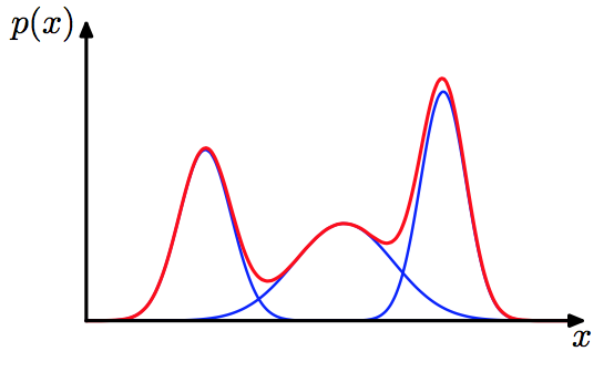With this assumption, we are equivalent to assuming a similarity between each client data, which is similar to finding the hidden IID components from non IID.

Next, let's look at how to design the function of this partition algorithm. In addition to the N required by the conventional Dirichlet partition algorithm_ clients,n_classes, \ (\ alpha \), etc. it also has a special n_ The clusters parameter indicates the number of mixed components. Let's look at the function prototype:

def split_dataset_by_labels(dataset, n_classes, n_clients, n_clusters, alpha, frac, seed=1234):

Let's explain the parameters of the function, where the dataset is torch utils. Dataset of type dataset, n_ Classes represents the number of sample classifications in the data set, n_ Clusters is the number of clusters (its meaning will be explained later. If it is set to - 1, it defaults to n_clusters=n_classes, which is equivalent to that each client is a cluster, that is, the mixed distribution assumption is abandoned). alpha is used to control the data diversity between clients. frac is the proportion of data sets used (the default is 1, that is, all data is used), Seed is the seed of the incoming random number. This function returns an_ Client a list consisting of a list of sample indexes required by a client_idcs.

Next, let's look at the content of this function. The content of this function can be summarized as follows: first group all categories into n_clusters: clusters; Then for each cluster c, the samples are divided into different clients (the number of samples for each client is determined according to the dirichlet distribution).

First, we judge n_ If the number of clusters is - 1, each cluster corresponds to a data class by default:

    if n_clusters == -1:
        n_clusters = n_classes

Then divide the disrupted tag set \ (\ {0,1,...,n\_classes-1 \} \) into n_clusters are independent and identically distributed clusters.

    all_labels = list(range(n_classes))
    np.random.shuffle(all_labels)
    def iid_divide(l, g):
        """
        Will list`l`Divided into`g`Independent identically distributed group(In fact, it is directly divided)
        each group All have `int(len(l)/g)` perhaps `int(len(l)/g)+1` Elements
        Return by different groups List of components
        """
        num_elems = len(l)
        group_size = int(len(l) / g)
        num_big_groups = num_elems - g * group_size
        num_small_groups = g - num_big_groups
        glist = []
        for i in range(num_small_groups):
            glist.append(l[group_size * i: group_size * (i + 1)])
        bi = group_size * num_small_groups
        group_size += 1
        for i in range(num_big_groups):
            glist.append(l[bi + group_size * i:bi + group_size * (i + 1)])
        return glist
    clusters_labels = iid_divide(all_labels, n_clusters)

Then create a dictionary with key as label and value as cluster id(group_idx) according to the above clusters_labels,

    label2cluster = dict()  # maps label to its cluster
    for group_idx, labels in enumerate(clusters_labels):
        for label in labels:
            label2cluster[label] = group_idx

Then get the index of the data set

    data_idcs = list(range(len(dataset)))

After that, we

    # Record the vector of the size of each cluster
    clusters_sizes = np.zeros(n_clusters, dtype=int)
    # Store the data index corresponding to each cluster
    clusters = {k: [] for k in range(n_clusters)}
    for idx in data_idcs:
        _, label = dataset[idx]
        # First find the id of the cluster from the label of the sample data
        group_id = label2cluster[label]
        # Then add the size of the corresponding cluster + 1
        clusters_sizes[group_id] += 1
        # Add the sample index to the list corresponding to its cluster
        clusters[group_id].append(idx)

    # Disrupt the sample index list corresponding to each cluster
    for _, cluster in clusters.items():
        rng.shuffle(cluster)

Next, we set the number of samples for each cluster according to the Dirichlet distribution.

    # Record the number of samples of client s from each cluster
    clients_counts = np.zeros((n_clusters, n_clients), dtype=np.int64) 

    # Traverse each cluster
    for cluster_id in range(n_clusters):
        # Each client in each cluster is given a weight that satisfies the dirichlet distribution
        weights = np.random.dirichlet(alpha=alpha * np.ones(n_clients))
        # np.random.multinomial means to roll dice clusters_sizes[cluster_id] times, and the weights on each client are weights in turn
        # This function returns the number of times it falls on each client, which corresponds to the number of samples each client should receive
        clients_counts[cluster_id] = np.random.multinomial(clusters_sizes[cluster_id], weights)

    # Prefix (accumulate) the counting times of each client on each cluster,
    # It is equivalent to the subscript of the sample dividing point divided according to the client in each cluster
    clients_counts = np.cumsum(clients_counts, axis=1)

Then, according to the sample situation of each client in each cluster (we have obtained the subscript of the sample dividing point divided according to the client in each cluster), we combine and summarize the sample situation of each client.

    def split_list_by_idcs(l, idcs):
        """
        Will list`l` Divided into length `len(idcs)` Sublist of
        The first`i`Sub list from subscript `idcs[i]` To subscript`idcs[i+1]`
        (Subscript 0 to subscript`idcs[0]`Sub list of (calculated separately)
        Returns a list consisting of multiple sub lists
        """
        res = []
        current_index = 0
        for index in idcs: 
            res.append(l[current_index: index])
            current_index = index

        return res
    
    clients_idcs = [[] for _ in range(n_clients)]
    for cluster_id in range(n_clusters):
        # cluster_split is the sample divided by client in a cluster
        cluster_split = split_list_by_idcs(clusters[cluster_id], clients_counts[cluster_id])

        # Add up the samples of each client
        for client_id, idcs in enumerate(cluster_split):
            clients_idcs[client_id] += idcs

Finally, we return the sample index corresponding to each client:

    return clients_idcs

Next, we call this function on EMNIST dataset for testing and visual rendering. We set the number of client s \ (N=10 \), the parameter vector \ (\ bm{\alpha} \) of Dirichlet probability distribution satisfies \ (\ alpha_i=0.4,\space i=1,2,...N \), and the number of mixed components is 3:

import torch
from torchvision import datasets
import numpy as np
import matplotlib.pyplot as plt

torch.manual_seed(42)

if __name__ == "__main__":

    N_CLIENTS = 10
    DIRICHLET_ALPHA = 1
    N_COMPONENTS = 3

    train_data = datasets.EMNIST(root=".", split="byclass", download=True, train=True)
    test_data = datasets.EMNIST(root=".", split="byclass", download=True, train=False)
    n_channels = 1


    input_sz, num_cls = train_data.data[0].shape[0],  len(train_data.classes)


    train_labels = np.array(train_data.targets)

    # Note that the number of samples of different label s of each client is different, so as to achieve non IID division
    client_idcs = split_dataset_by_labels(train_data, num_cls, N_CLIENTS, N_COMPONENTS, DIRICHLET_ALPHA)


    # Display the data distribution of different label s of different client s
    plt.figure(figsize=(20,3))
    plt.hist([train_labels[idc]for idc in client_idcs], stacked=True, 
            bins=np.arange(min(train_labels)-0.5, max(train_labels) + 1.5, 1),
            label=["Client {}".format(i) for i in range(N_CLIENTS)], rwidth=0.5)
    plt.xticks(np.arange(num_cls), train_data.classes)
    plt.legend()
    plt.show()

The final visualization results are as follows:

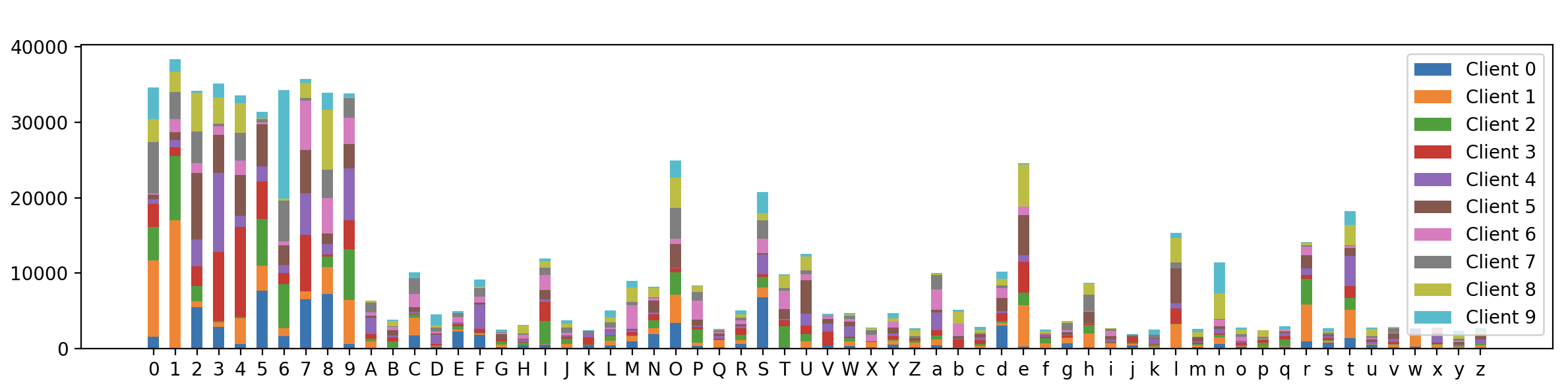
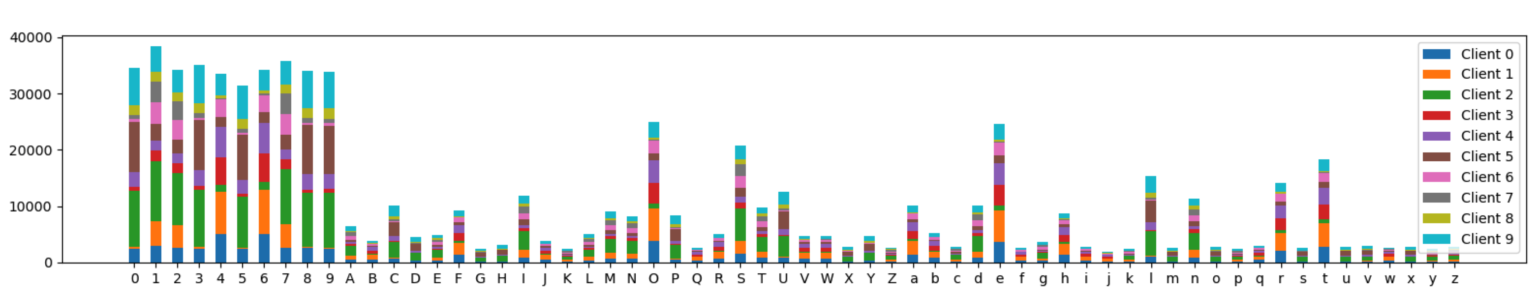It can be seen that although the distribution of 62 category labels on different clients is different, the data distribution between each client is more similar than the following sample partition algorithm based entirely on Dirichlet, which proves that our mixed distribution sample partition algorithm is effective.

reference resources

• [1] McMahan B, Moore E, Ramage D, et al. Communication-efficient learning of deep networks from decentralized data[C]//Artificial intelligence and statistics. PMLR, 2017: 1273-1282.

• [2] Marfoq O, Neglia G, Bellet A, et al. Federated multi-task learning under a mixture of distributions[J]. Advances in Neural Information Processing Systems, 2021, 34.