dichotomy
The dichotomy is a simple and effective numerical iteration algorithm for an interval
[
a
,
b
]
\left[a,b\right]
The continuous function fx on [a,b], if it satisfies
f
(
a
)
⋅
f
(
b
)
<
0
f(a)\cdot f(b)<0
F(a)f(b)<0, then fx in
[
a
,
b
]
\left[a,b\right]
There must be a root on [a,b], set the split point
x
0
=
(
a
+
b
)
/
2
x_0=\left(a+b\right)/2
x0 = (a+b)/2 divides the intervals equally
[
a
,
x
0
]
\left[a,x_0\right]
[a,x0] and
[
x
0
,
b
]
\left[x_0,b\right]
[x0, b], calculate
f
(
a
)
⋅
f
(
x
0
)
f\left(a\right)\cdot f\left(x_0\right)
f(a)⋅f(x0),
f
(
x
0
)
⋅
f
(
b
)
f\left(x_0\right)\cdot f\left(b\right)
f(x0)f(b), then the root must be in one of the intervals, repeat the process N times until the interval in which the root is located is long enough to stop iteration. Although the dichotomy guarantees final convergence near the root, it also has an extreme case where the root happens to be in another interval in each iteration, so the time complexity is
O
=
log
2
(
N
)
O=\log_2{\left(N\right)}
O=log2 (N). The process of dichotomy is shown in the following figure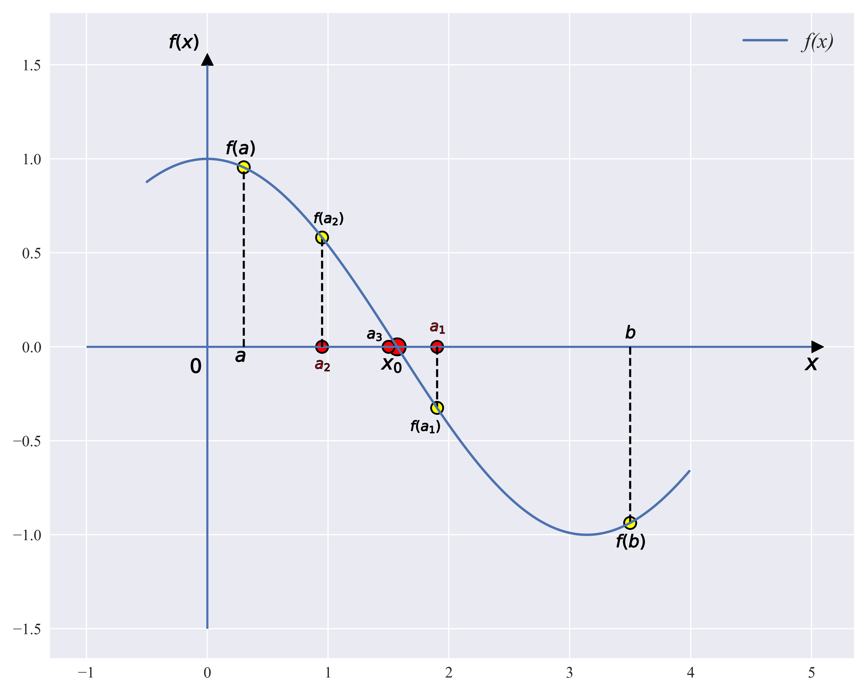
- Source code
import math
import numpy as np
import matplotlib.pyplot as plt

x = np.arange(-0.5, 4, 0.01)
y = np.cos(x)
plt.figure(figsize=(10, 8))
plt.plot(x, y,label="f(x)",linewidth=2)
plt.vlines(x=0, ymin=-1.5, ymax=1.5)
plt.hlines(y=0, xmin=-1, xmax=5)
#plt.xlabel("x")
#plt.ylabel("cos(x)")
plt.vlines(x=0.3, ymin=0, ymax=cos(0.3), linestyle="--", color="black")
plt.scatter(0.3, cos(0.3), c = 'yellow', marker = 'o',s=100, edgecolors="black",alpha = 1, linewidths = 1.5)
plt.vlines(x=3.5, ymin=0, ymax=cos(3.5), linestyle="--", color="black")
plt.scatter(3.5, cos(3.5), c = 'yellow', marker = 'o',s=100, edgecolors="black",alpha = 1, linewidths = 1.5)
plt.scatter(0.27, -0.05, c = 'black', marker = '$a$', s=80, alpha = 1, linewidths = 0.5)
plt.scatter(3.5, 0.08, c = 'black', marker = '$b$', s=120, alpha = 1, linewidths = 0.5)
plt.scatter(0.27, cos(0.3)+0.1, c = 'black', marker = '$f(a)$', s=580, alpha = 1, linewidths = 0.5)
plt.scatter(3.5, cos(3.5)-0.1, c = 'black', marker = '$f(b)$', s=580, alpha = 1, linewidths = 0.5)
plt.scatter(np.pi/2-0.05, cos(np.pi/2)-0.1, c = 'black', marker = '$x_0$', s=280, alpha = 1, linewidths = 0.5)
plt.scatter(np.pi/2, cos(np.pi/2), c = 'red', marker = 'o', s=200, edgecolors="black",alpha = 1,linewidths = 1.5)

plt.scatter((0.3+3.5)/2, 0, c = 'red', marker = 'o', s=100, edgecolors="black", alpha = 1, linewidths = 1.5)
plt.scatter((0.3+3.5)/2, 0+0.1, c = 'red', marker = '$a_1$', s=150, edgecolors="black", alpha = 1, linewidths = 0.5)
plt.scatter((0.3+3.5)/2-0.1, cos((0.3+3.5)/2)-0.1, c = 'black', marker = '$f(a_1)$', s=600, edgecolors="black", alpha = 1, linewidths = 0.5)
plt.scatter((0.3+3.5)/2, cos((0.3+3.5)/2), c = 'yellow', marker = 'o', s=100, edgecolors="black", alpha = 1, linewidths = 1.5)
plt.vlines(x=(0.3+3.5)/2, ymin=0, ymax=cos((0.3+3.5)/2), linestyle="--",color="black")
plt.scatter((0.3+3.5)/4, 0, c = 'red', marker = 'o', s=100, edgecolors="black", alpha = 1, linewidths = 1.5)
plt.scatter((0.3+3.5)/4, 0-0.1, c = 'red', marker = '$a_2$', s=150, edgecolors="black", alpha = 1, linewidths = 0.5)
plt.vlines(x=(0.3+3.5)/4, ymin=0, ymax=cos((0.3+3.5)/4), linestyle="--", color="black")
plt.scatter((0.3+3.5)/4, cos((0.3+3.5)/4), c = 'yellow', marker = 'o', s=100, edgecolors="black", alpha = 1, linewidths = 1.5)
plt.scatter((0.3+3.5)/4+0.05, cos((0.3+3.5)/4)+0.1, c = 'black', marker = '$f(a_2)$', s=600, edgecolors="black", alpha = 1, linewidths = 0.5)
plt.scatter(1.5, 0, c='red', marker = 'o', s=100, edgecolors="black", alpha = 1, linewidths = 1.5)
plt.scatter(1.38, 0.06, c='black', marker = '$a_3$', s=150, edgecolors="black", alpha = 1, linewidths = 0.5)
plt.scatter(-0.1, -0.1, c='black', marker = '$0$', s=150, edgecolors="black", alpha = 1, linewidths = 0.5)
plt.scatter(5.05, 0, c='black', marker = '>', s=100, edgecolors="black", alpha = 1, linewidths = 0.5)
plt.scatter(0, 1.53, c='black', marker = '^', s=100, edgecolors="black", alpha = 1, linewidths = 0.5)
plt.scatter(-0.2, 1.62, c='black', marker = '$f(x)$', s=600, edgecolors="black", alpha = 1, linewidths = 0.5)
plt.scatter(5.0, -0.09, c='black', marker = '$x$', s=130, edgecolors="black", alpha = 1, linewidths = 0.5)
plt.yticks(fontstyle = "normal", fontproperties = 'Times New Roman', size = 13)
plt.xticks(fontstyle = "normal", fontproperties = 'Times New Roman', size = 13)
#plt.xlabel('x', fontdict=fontdict_ita)
#plt.ylabel("f (x)", fontdict=fontdict_ita)
plt.legend(prop=fontdict_ita)
plt.tight_layout()
plt.show()
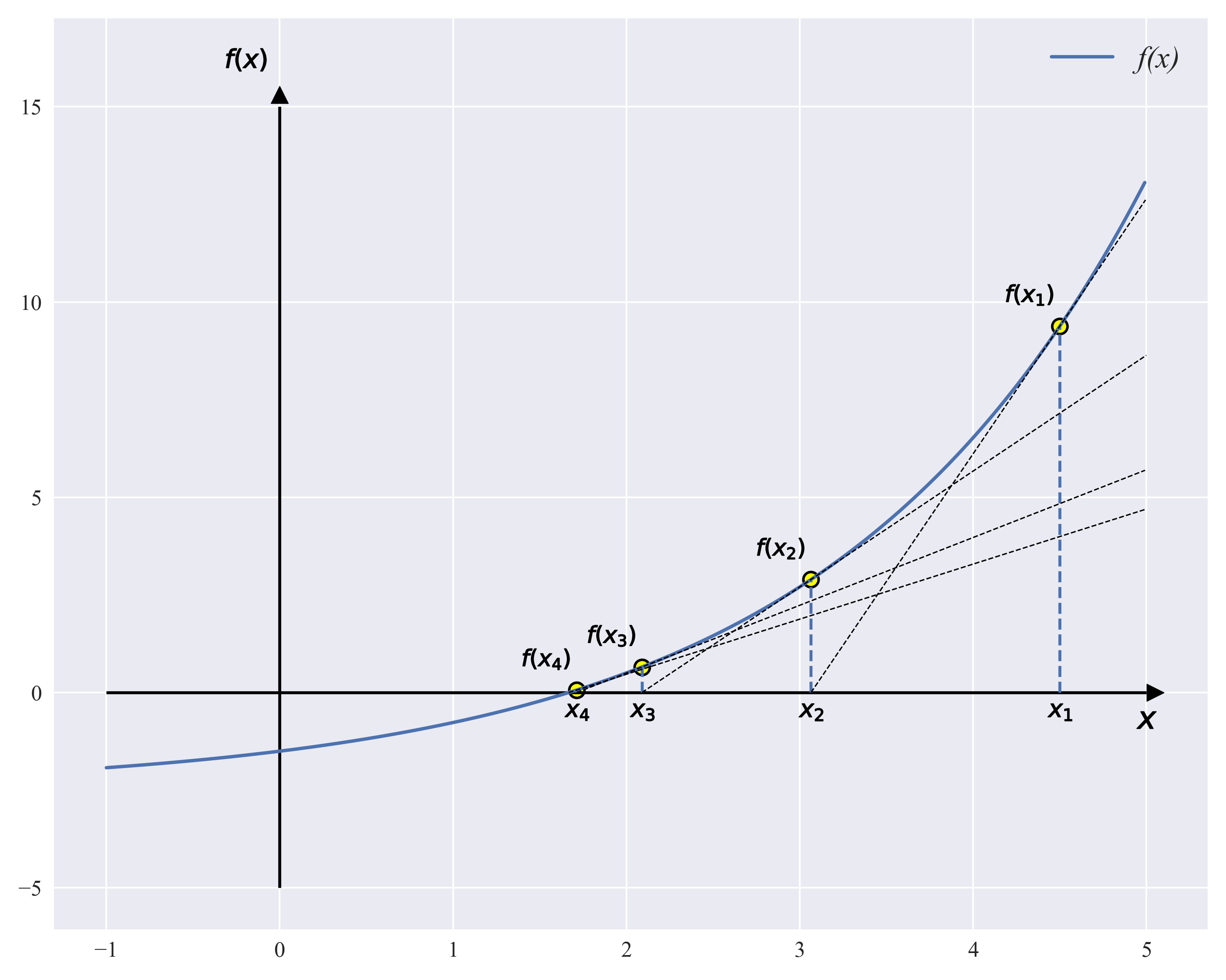
Newton iteration method
Newton-Raphson iteration algorithm, also called Newton method, is the most familiar and widely used numerical calculation method. Newton's iteration method is one of the important methods to find the root of the equation. Its greatest advantage is in the equation
f
(
x
)
=
0
f\left(x\right)=0
The algorithm can also be used to find the multiple and complex roots of the equation. In this case, the linear convergence can be changed into superlinear convergence by some methods. In addition, this method is widely used in computer programming. If the saddle point equation is
f
(
t
)
f\left(t\right)
f(t),
r
r
r is the root of the equation, select
x
0
x_0
x0 as initial iteration value, through point
(
x
0
,
f
(
x
0
)
)
\left(x_0,f\left(x_0\right)\right)
(x0, f(x0)) curve
f
(
t
)
f\left(t\right)
Tangent of f(t)
L
L
L, then the expression with L according to the point slant is
L
:
y
=
f
(
x
0
)
+
f
′
(
x
0
)
(
x
−
x
0
)
L:y=f(x_0)+f'(x_0)(x-x_0)
L:y=f(x0)+f′(x0)(x−x0)
The tangent intersects the x-axis
x
1
=
x
0
−
f
(
x
0
)
f
′
(
x
0
)
x_1=x_0-\frac{f(x_0)}{f'(x_0)}
x1=x0−f′(x0)f(x0)
Transit Point
(
x
1
,
f
(
x
1
)
)
\left(x_1,f\left(x_1\right)\right)
(x1, f(x1)) do the curve again
f
(
x
)
f\left(x\right)
Tangent of f(x)
x
2
x_2
x2, repeat the above process
N
N
N times until
x
n
+
1
−
x
n
≤
ε
x_{n+1}-x_n\le\varepsilon
xn+1 xn < or equal to ε End iteration. A large number of literatures have shown that if the root of the equation exists in isolation, there is a neighborhood near the root within which the initial iteration values must eventually converge to the root of the equation. The following figure shows the calculation of Newton's method
x = np.arange(-1, 5, 0.01)
k = 0.55
def f(x):
    return np.exp(k*x)-2.5
def d_f(x):
    return k*exp(k*x)
x0 = 4.5

plt.figure(figsize=(10, 8))
plt.plot(x, f(x), label="f(x)", linewidth=2)
plt.vlines(x=0, ymin=-5, ymax=15, color="black")
plt.hlines(y=0, xmin=-1, xmax=5, color="black")
n=5
for i in range(1, n):
    #cut = -f(x1)*(x1 - x0)/(f(x1) - f(x0)) + x1
    x1 = x0 - f(x0)/d_f(x0)
    xx = np.arange(x1, 5, 0.01)
    yy = f(x0) + d_f(x0)*(xx - x0)
    plt.plot(xx, yy, color="black", linestyle="--", linewidth=0.8)
    plt.scatter(x0, f(x0), c='yellow', marker = 'o', s=size_o , edgecolors="black", alpha = 1, linewidths = 1.5)
    plt.scatter(x0 - 0.18, f(x0) + 0.8, c='black', marker=marker_fx[i-1], s=800 , edgecolors="black", alpha = 1, linewidths = 0.5)
    plt.scatter(x0, -0.5, c='black', marker = marker_x[i-1], s=size_x , edgecolors="black", alpha = 1, linewidths = 0.5)
    plt.vlines(x=x0, ymin=0, ymax=f(x0), linestyle="--")
    x0 = x1
    x1 = cut

plt.yticks(fontstyle = "normal", fontproperties = 'Times New Roman', size = 13)
plt.xticks(fontstyle = "normal", fontproperties = 'Times New Roman', size = 13)
plt.scatter(5.05, 0, c='black', marker = '>', s=100, edgecolors="black", alpha = 1, linewidths = 0.5)
plt.scatter(0, 15.3, c='black', marker = '^', s=100, edgecolors="black", alpha = 1, linewidths = 0.5)
plt.scatter(-0.2, 16.2, c='black', marker = '$f(x)$', s=600, edgecolors="black", alpha = 1, linewidths = 0.5)
plt.scatter(5.0, -0.7, c='black', marker = '$x$', s=130, edgecolors="black", alpha = 1, linewidths = 0.5)
plt.legend(prop=fontdict_ita)
plt.tight_layout()
plt.show()
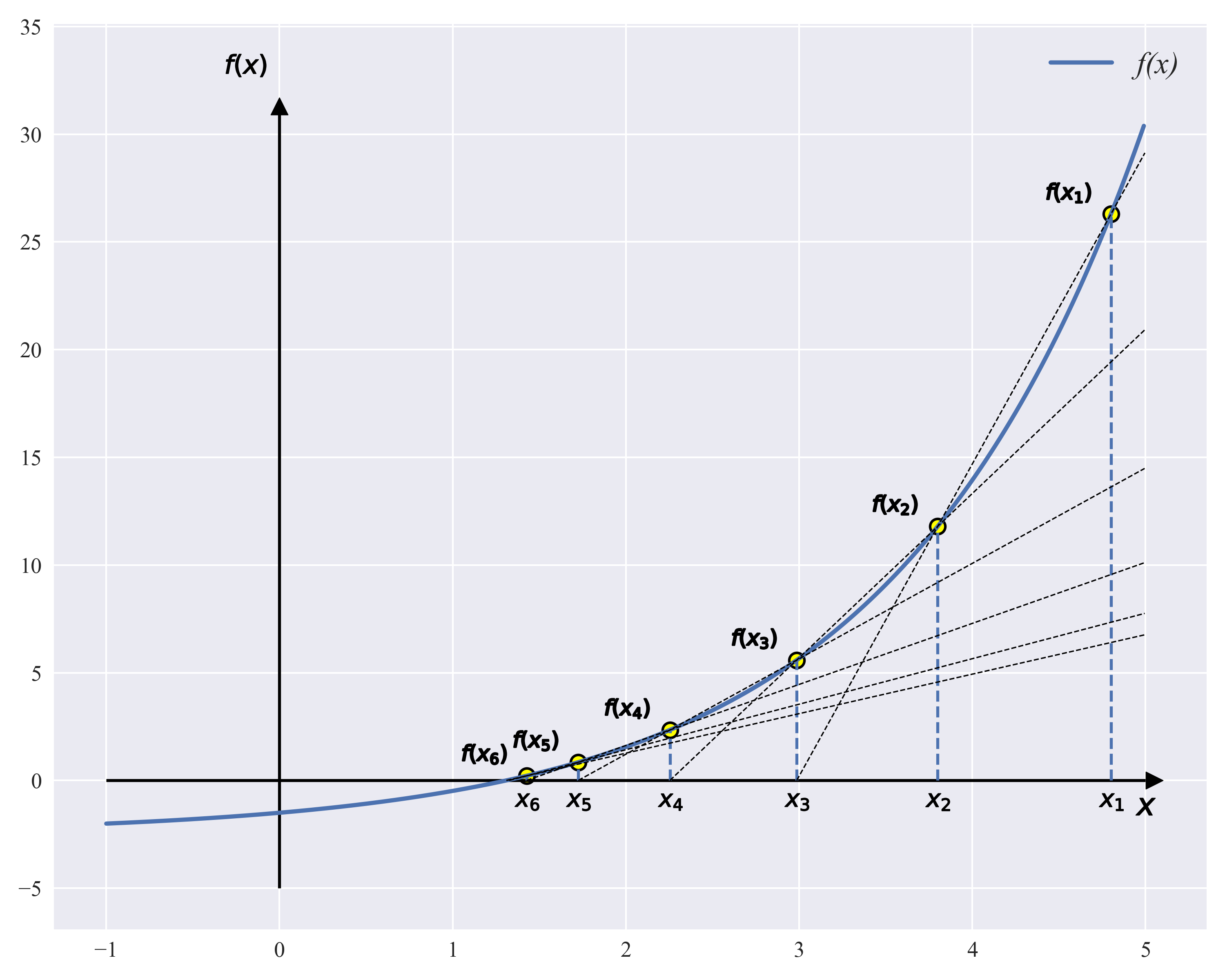
Secant method
The secant method is an improvement of Newton's method. The idea is to replace the tangent of the equation solved in Newton's method with the secant, and then use the intersection of the Secant and the x-axis as the approximate solution of the root. Given function
f
(
x
)
f\left(x\right)
f(x) and two points on a function
(
x
1
,
f
(
x
1
)
)
\left(x_1,f\left(x_1\right)\right)
(x1,f(x1)),
(
x
2
,
f
(
x
2
)
)
\left(x_2,f\left(x_2\right)\right)
(x2, f(x2))), then secant L is given by the two-point formula
y
−
f
(
x
1
)
=
f
(
x
1
)
−
f
(
x
0
)
x
1
−
x
0
(
x
−
x
1
)
y-f(x_1)=\frac{f(x_1)-f(x_0)}{x_1-x_0}(x-x_1)
y−f(x1)=x1−x0f(x1)−f(x0)(x−x1)
At this point L and
x
x
x-axis intersects at
x
2
x_2
x2 dots, redone
x
1
x_1
x1,
x
2
x_2
The secant of x2 intersects the transverse axis
x
3
x_3
x3, repeat the above process
N
N
N times until
x
n
−
x
n
−
1
x_n-x_{n-1}
Xn xn 1 converges to the given error limit. Unlike Newton's method, secant method requires two initial iteration points to be given in advance. The algorithm process is shown in the following figure
x = np.arange(-1, 5, 0.01)
k = 0.7

def f(x):
    return np.exp(k*x)-2.5
def d_f(x):
    return k * exp(k * x)


x0 = 4.8; f0 = f(x0)
x1 = 3.8; f1 = f(x1)
n = 7

plt.figure(figsize=(10, 8))
plt.plot(x, f(x), linewidth=2.5, label="f(x)")
plt.vlines(x=0, ymin=-5, ymax=f(max(x))+1, color="black")
plt.hlines(y=0, xmin=-1, xmax=5, color="black")

marker_fx = []
marker_x = []
for i in range(1, n):
    lab = "$f(x_" + str(i) + ")$"
    lab2 = "$x_" + str(i) + "$"
    marker_fx.append(lab)
    marker_x.append(lab2)

for i in range(1, n):
    cut = -f(x1)*(x1 - x0)/(f(x1) - f(x0)) + x1
    xx = np.arange(cut, 5, 0.01)
    yy = (xx - x1)*((f(x1) - f(x0))/(x1 - x0)) + f(x1)
    plt.plot(xx, yy, color="black", linestyle="--", linewidth=0.8)
    plt.scatter(x0, f(x0), c='yellow', marker = 'o', s=size_o , edgecolors="black", alpha = 1, linewidths = 1.5)
    plt.scatter(x0 - 0.25, f(x0) + 1, c='black', marker=marker_fx[i-1], s=700 , edgecolors="black", alpha = 1, linewidths = 1)
    plt.scatter(x0, -1.0, c='black', marker = marker_x[i-1], s=size_x , edgecolors="black", alpha = 1, linewidths = 0.5)
    plt.vlines(x=x0, ymin=0, ymax=f(x0), linestyle="--")
    x0 = x1
    x1 = cut

plt.yticks(fontstyle = "normal", fontproperties = 'Times New Roman', size = 13)
plt.xticks(fontstyle = "normal", fontproperties = 'Times New Roman', size = 13)
plt.scatter(5.05, 0, c='black', marker = '>', s=100, edgecolors="black", alpha = 1, linewidths = 0.5)
plt.scatter(0, 31.3, c='black', marker = '^', s=100, edgecolors="black", alpha = 1, linewidths = 0.5)
plt.scatter(-0.2, 33.2, c='black', marker = '$f(x)$', s=600, edgecolors="black", alpha = 1, linewidths = 0.5)
plt.scatter(5.0, -1.2, c='black', marker = '$x$', s=130, edgecolors="black", alpha = 1, linewidths = 0.5)
plt.legend(prop=fontdict_ita)
plt.tight_layout()
plt.show()
secant method
Chord truncation can be seen as an extension of dichotomy. if
f
(
t
)
f\left(t\right)
f(t) in the zone
[
a
,
b
]
\left[a,b\right]
Continuous on [a,b] and f
(
a
)
⋅
f
(
b
)
<
0
\left(a\right)\cdot f\left(b\right)<0
(a) f(b)<0, then
[
[
a
,
b
]
[\left[a,b\right]
[[a,b] is a root interval. Do it now
f
(
t
)
f(t)
f(t) over A
(
a
,
f
(
a
)
)
(a,f(a))
(a,f(a)),
B
(
b
,
f
(
b
)
)
B\left(b,f\left(b\right)\right)
The chord AB of point B(b,f(b)) has a
L
:
y
=
b
−
x
b
−
a
f
(
a
)
+
x
−
a
b
−
a
f
(
b
)
L:y=\frac{b-x}{b-a}f(a)+\frac{x-a}{b-a}f(b)
L:y=b−ab−xf(a)+b−ax−af(b)
Chord AB intersects x-axis
x
=
a
−
f
(
a
)
f
(
b
)
−
f
(
a
)
(
b
−
a
)
x=a-\frac{f(a)}{f(b)-f(a)}(b-a)
x=a−f(b)−f(a)f(a)(b−a)
And as
f
(
t
)
f\left(t\right)
f(t) in
[
a
,
b
]
\left[a,b\right]
Root on [a,b]. Repeat the process until the root interval is small enough to stop the iteration. Unlike the dichotomy, the new interval obtained by the chord truncation method may not be equally divided each time, and the chord is made continuously after the B-point is fixed, which makes the search faster than the dichotomy. The process of chord truncation is shown in the following figure
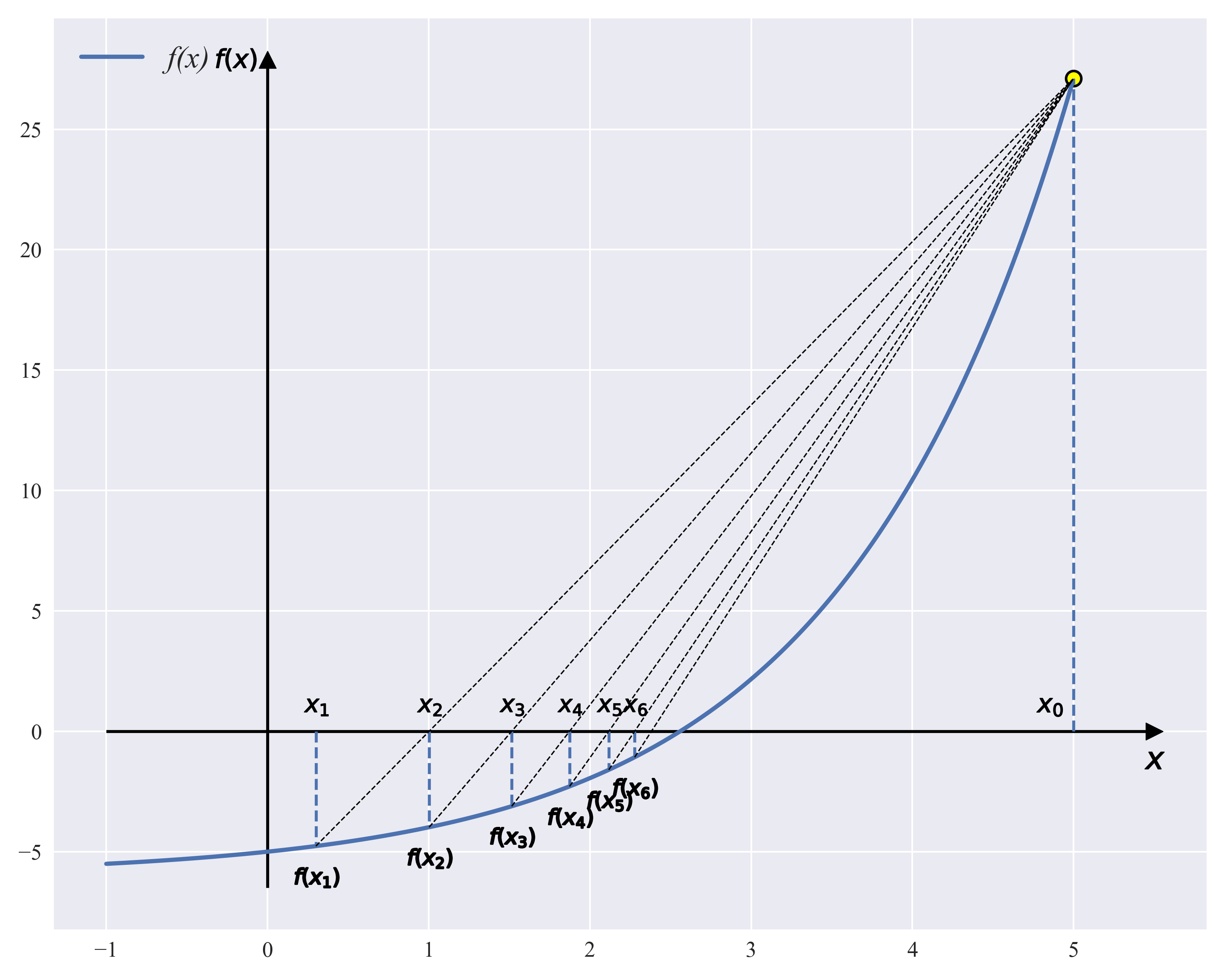
The intersection of the line L and the transverse axis obtained by the visible chord truncation always lies on the left side of the root, making it
f
(
x
n
)
⋅
f
(
x
0
)
<
0
f\left(x_n\right)\cdot f\left(x_0\right)<0
f(xn)f(x0)<0 can always be satisfied.
x = np.arange(-1, 5, 0.01)
k = 0.7

def f(x):
    return np.exp(k*x)-6
def d_f(x):
    return k * exp(k * x)


x0 = 5.0; f0 = f(x0)
x1 = 0.3; f1 = f(x1)
n = 7

plt.figure(figsize=(10, 8))
plt.plot(x, f(x), linewidth=2.5, label="f(x)")
plt.vlines(x=0, ymin=f(min(x))-1, ymax=f(max(x))+1, color="black")
plt.hlines(y=0, xmin=-1, xmax=x0+0.5, color="black")
plt.vlines(x=x0, ymin=0, ymax=f(x0), linestyle="--")


marker_fx = []
marker_x = []
for i in range(1, n):
    lab = "$f(x_" + str(i) + ")$"
    lab2 = "$x_" + str(i) + "$"
    marker_fx.append(lab)
    marker_x.append(lab2)

for i in range(1, n):
    cut = x1 - (x0-x1)*(f(x1))/(f(x0)-f(x1))
    xx = np.arange(x1, 5, 0.01)
    yy = f(x1)*(x0-xx)/(x0-x1) + f(x0)*(xx-x1)/(x0-x1)
    plt.plot(xx, yy, color="black", linestyle="--", linewidth=0.8)
    plt.scatter(x1, f(x1)-1.3, c='black', marker=marker_fx[i-1], s=700 , edgecolors="black", alpha = 1, linewidths = 1) #fx
    plt.scatter(x1, 1.0, c='black', marker = marker_x[i-1], s=size_x , edgecolors="black", alpha = 1, linewidths = 0.5)   #x
    plt.vlines(x=x1, ymin=0, ymax=f(x1), linestyle="--")
    #x0 = x1
    x1 = cut

plt.yticks(fontstyle = "normal", fontproperties = 'Times New Roman', size = 13)
plt.xticks(fontstyle = "normal", fontproperties = 'Times New Roman', size = 13)
plt.scatter(x0, f(x0), c='yellow', marker = 'o', s=size_o , edgecolors="black", alpha = 1, linewidths = 1.5)
plt.scatter(x0+0.5, 0, c='black', marker = '>', s=100, edgecolors="black", alpha = 1, linewidths = 0.5)
plt.scatter(0, f(max(x))+1, c='black', marker = '^', s=100, edgecolors="black", alpha = 1, linewidths = 0.5)
plt.scatter(-0.2, f(max(x))+1, c='black', marker = '$f(x)$', s=600, edgecolors="black", alpha = 1, linewidths = 0.5)
plt.scatter(x0+0.5, -1.2, c='black', marker = '$x$', s=130, edgecolors="black", alpha = 1, linewidths = 0.5)
plt.scatter(4.85, 1, c='black', marker = '$x_0$', s=230, edgecolors="black", alpha = 1, linewidths = 0.5)
plt.legend(prop=fontdict_ita)
plt.tight_layout()
plt.show()
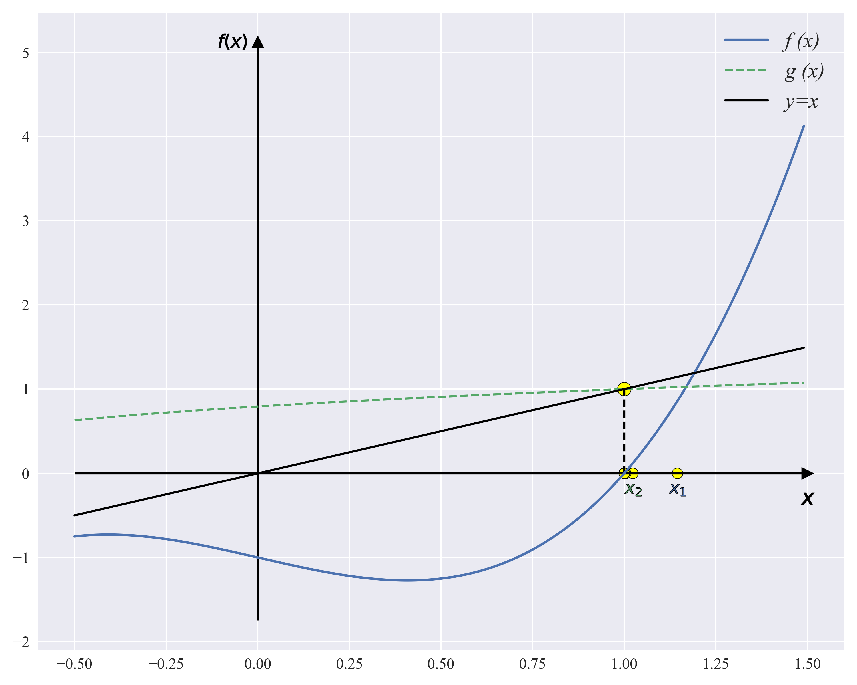
Fixed Point Method
The fixed point iteration method is also called simple iteration. The Newton method that we commonly use is a special form of fixed point iteration algorithm. To solve the equation
f
(
x
)
=
0
f\left(x\right)=0
f(x)=0, first set the
f
(
x
)
f\left(x\right)
f(x) to
x
=
g
(
x
)
x=g\left(x\right)
x=g(x) and needs to be satisfied
∣
g
(
x
)
∣
<
1
\left|g\left(x\right)\right|<1
_g(x)<1, given the initial value of the iteration
x
0
x_0
x0, circular calculation
x
n
+
1
=
g
(
x
n
)
x_{n+1}=g\left(x_n\right)
xn+1 =g(xn) until
x
n
+
1
−
x
n
x_{n+1}-x_n
xn+1 xn is less than the set error limit
ε
\varepsilon
ε. However, this method does not guarantee convergence near the root, on the contrary, if the initial value is too far from the root, the result will diverge. For example, when we want to solve an equation
2
x
3
−
x
−
1
=
0
2x^3-x-1=0
Root of 2x3_x_1=0, equation
f
(
x
)
=
0
f\left(x\right)=0
f(x)=0 is not unique and can be converted to
x
=
2
x
3
−
1
x=2x^3-1
x=2x3_1 or
x
=
(
(
x
+
1
)
/
2
)
1
/
3
x=\left(\left(x+1\right)/2\right)^{1/3}
x=((x+1)/2)1/3. From a geometric point of view, the problem of solving roots is transformed into a solution
y
=
x
y=x
y=x and
g
(
x
)
g\left(x\right)
g(x) intersection problem. The approximation of the root can be obtained by continuously calculating the iteration. The following figure shows the process of the fixed point iteration algorithm.
import numpy as np
x = np.arange(-5, 5, 0.01)
x0 = 2
def f(x):
    return 2*x**3-x-1

def g(x):
    return pow((x+1)/2,1/3)
def f2(x):
    return x
xk = []
for k in range(20):
    xk1 = g(x0)
    xk.append(g(x0))
    x0 = xk1
import matplotlib.pyplot as plt
fontdict_nor = {'family' : 'Times New Roman', 'size': 18, "style":"normal"}
fontdict_ita = {'family' : 'Times New Roman', 'size': 18, "style":"italic"}
plt.style.use("seaborn")
plt.style.use("seaborn")
x = np.arange(-0.5, 1.5, 0.01)

plt.figure(figsize=(10, 8))

n = len(xk)
marker_fx = []
marker_x = []
for i in range(1, n):
    lab = "$f(x_" + str(i) + ")$"
    lab2 = "$x_" + str(i) + "$"
    marker_fx.append(lab)
    marker_x.append(lab2)


plt.plot(x, f(x), label="f (x)", linewidth=2)
plt.plot(x, g(x), label="g (x)", linestyle="--")
plt.plot(x, f2(x),label="y=x", color="black")

plt.vlines(x=0, ymin=f(min(x))-1, ymax=f(max(x))+1, color="black")
plt.hlines(y=0, xmin=-0.5, xmax=1.5, color="black")

for i in range(len(xk)):
    plt.scatter(xk[i], 0, c='yellow', marker = 'o', s=80, edgecolors="black", alpha = 1, linewidths = 0.5)

for i in range(2):
    plt.scatter(xk[i], -0.2, marker = marker_x[i], s=200, edgecolors="black", alpha = 1, linewidths = 0.5)

plt.yticks(fontstyle = "normal", fontproperties = 'Times New Roman', size = 13)
plt.xticks(fontstyle = "normal", fontproperties = 'Times New Roman', size = 13)

plt.scatter(x0+0.5, 0, c='black', marker = '>', s=100, edgecolors="black", alpha = 1, linewidths = 0.5)
plt.scatter(0, f(max(x))+1, c='black', marker = '^', s=100, edgecolors="black", alpha = 1, linewidths = 0.5)
plt.scatter(-0.07, f(max(x))+1, c='black', marker = '$f(x)$', s=600, edgecolors="black", alpha = 1, linewidths = 0.5)
plt.scatter(1.5, -0.3, c='black', marker = '$x$', s=130, edgecolors="black", alpha = 1, linewidths = 0.5)
plt.scatter(xk[-1], f2(xk[-1]), c='yellow', marker = 'o', s=130, edgecolors="black", alpha = 1, linewidths = 0.5)


plt.vlines(x=xk[-1], ymin=0, ymax=f2(xk[-1]), color="black", linestyle="--")

plt.legend(prop=fontdict_ita)
plt.tight_layout()
plt.show()