Baidu cloud link of the file used in this article:

Link: https://pan.baidu.com/s/15-qbrbtRs4frup24Y1i5og 
Extraction code: pm2c 

linear prediction

Assuming that a set of data conforms to a linear law, we can predict the data that will appear in the future

a  b  c  d  e  f  g  h  ....
ax + by + cz = d
bx + cy + dz = e
cx + dy + ez = f

In fact, the only way to solve the nonlinear equations is to use the API matrix fitting principle to solve the set of nonlinear equations, which provides a simple solution to the nonlinear equations:

x = np.linalg.lstsq(A, B)

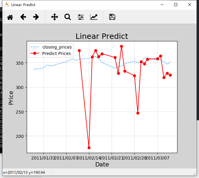
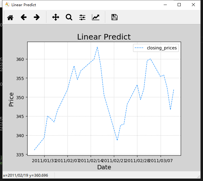
Look at the data. One part is the date, and the other part is the closing price of the day. Draw these data. As shown in the figure: it can be seen that there is a fluctuation in the closing price every day. Then we make a prediction according to this data. First of all, it is stated that this prediction is only to demonstrate the relevant methods of data processing and cannot be used in the practical application of stock speculation.

Sort out the ternary first-order equations and realize the linear prediction based on the linear model

The following code is a prediction process:

  first, calculate the amount of data to be predicted according to the existing data. Because it is a prediction, it needs a certain basis. Here we use the data of the first 10 days to predict the results of the next day, so N=5, pred_vals is an array of all the predicted results.

N = 5
pred_vals = np.zeros(closing_prices.size-2*N+1)

   then start the prediction. During each prediction, the data of 10 days are constructed into a 5 * 5 matrix, and the data of 6 to 10 days are used as the output of the first five days, which is equivalent to listing a five element one-time equation system. In fact, this construction method has no basis, but is designed by myself. Later, I will know if I do data processing and write algorithms, The algorithms are designed by ourselves. Whether the effect is good or not can only depend on the results.

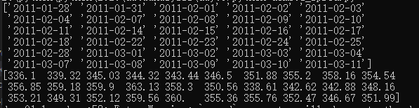
for i in range(pred_vals.size):
	A = np.zeros((N, N))
	for j in range(N):
		A[j,] = closing_prices[j+i:i+j+N]
	B = closing_prices[i+N:i+N*2]

   the solution equation here is actually matrix solution. In fact, it is to find the inverse matrix by Gauss Jordan elimination method, and then get the solution of x, that is, the transformation matrix. Then multiply the transformation matrix one by one with the corresponding matrix B to be predicted, and you can get the desired prediction result pred.

	x = np.linalg.lstsq(A, B)[0]
	pred = B.dot(x) # Point B multiplied by x [3] * x + [4] * y + [5] * Z
	pred_vals[i] = pred

Then take a look at the complete code and prediction results of the case: take a look at the results. Generally speaking, the predicted trend is still the same, but there will be some extreme value problems. Of course, this is only the simplest prediction.

"""
linear prediction
"""
import numpy as np
import matplotlib.pyplot as mp
import datetime as dt
import matplotlib.dates as md

# When numpy parses text, each string in the first column is
# Are passed to the function for processing, and the return value after processing is returned
# Convert to required M8[D] type
def dmy2ymd(dmy):
	dmy = str(dmy, encoding='utf-8')
	# Convert dmy to date object
	d = dt.datetime.strptime(dmy, '%d-%m-%Y')
	t = d.date()
	s = t.strftime('%Y-%m-%d')
	return s

# load file
dates, closing_prices = np.loadtxt(
	'../da_data/aapl.csv', delimiter=',', 
	usecols=(1,6), unpack=True, 
	dtype='M8[D], f8' , 
	converters={1:dmy2ymd})
# Draw closing price
mp.figure('Linear Predict', facecolor='lightgray')
mp.title('Linear Predict', fontsize=18)
mp.xlabel('Date', fontsize=14)
mp.ylabel('Price', fontsize=14)
mp.tick_params(labelsize=10)
mp.grid(linestyle=':')
# Set the master scale locator to Monday
ax = mp.gca()
ax.xaxis.set_major_locator(
	md.WeekdayLocator(byweekday=md.MO))
ax.xaxis.set_major_formatter(
	md.DateFormatter('%Y/%m/%d'))

# Change M8[D] to the date type recognized by matplotlib
dates = dates.astype(md.datetime.datetime)
mp.plot(dates, closing_prices, 
	color='dodgerblue', linewidth=1,
	linestyle='--', label='closing_prices')

# Sort out the ternary first-order equations and realize the linear prediction based on the linear model
N = 5

pred_vals = np.zeros(closing_prices.size-2*N+1)
# print(dates.shape)
for i in range(pred_vals.size):
	A = np.zeros((N, N))
	for j in range(N):
		A[j,] = closing_prices[j+i:i+j+N]
	# print(A)
	B = closing_prices[i+N:i+N*2]
	# print(B)
	x = np.linalg.lstsq(A, B)[0]
	print(x)
	pred = B.dot(x) # Point B multiplied by x [3] * x + [4] * y + [5] * Z
	pred_vals[i] = pred
# print(pred_vals)
# Draw forecast line chart
mp.plot(dates[2*N:], pred_vals[:-1], 'o-',
	color='red', label='Predict Prices')

mp.legend()
# Automatically format the date output of the x-axis
# mp.gcf().autofmt_xdate()
mp.show()