Author shivani46

Compile | Flin

introduce

The purpose of this paper is to show the process of using time series from data processing to constructing neural network and verifying results. As an example, the financial series is selected as completely random. Generally speaking, it is interesting if the traditional neural network architecture can capture the necessary patterns to predict the behavior of financial instruments.

The pipeline described in this article can be easily applied to any other data and other classification algorithms.

Data preparation for financial time series forecasting

For example, take the stock price of ordinary companies such as apple since 2005. It can be downloaded from Yahoo Finance in. csv format( https://finance.yahoo.com/quote/AAPL/history?period1=1104534000&period2=1491775200&interval=1d&filter=history&frequency=1d ).

Let's load the data and see what it looks like.

First, let's import the library we need to download:

import matplotlib.pylab as plt
import numpy as np
import pandas as pd

Now, just read the data to draw the graph. Don't forget to use [: – 1] to flip the data, because the CSV data is in reverse order, that is, from 2017 to 2005:

data = pd.read_csv('./data/AAPL.csv')[::-1]
close_price = data.ix[:, 'Adj Close'].tolist()
plt.plot(close_price)
plt.show()

It looks almost like a typical stochastic process, but we will try to solve the problem of predicting one day or more in advance. The problem of "prediction" must first be described closer to the problem of machine learning.

We can simply predict the change of stock price in the market - more or less - which will be a binary classification problem.

On the other hand, we can only predict the price value of the next day (or a few days later), or the price change of the next day compared with the previous day, or the logarithm of this difference - that is, we want to predict a number, which is a regression problem. However, when solving the regression problem, you will have to face the problem of data normalization, which we will consider now.

Whether in the case of classification or regression, we will try to predict the price trend (classification) or the value of change (regression) the next day with a certain time series window (for example, 30 days) as the entrance.

The main problem with financial time series is that they are not stable at all.

The expected value, variance, average maximum and minimum values change over time in the window.

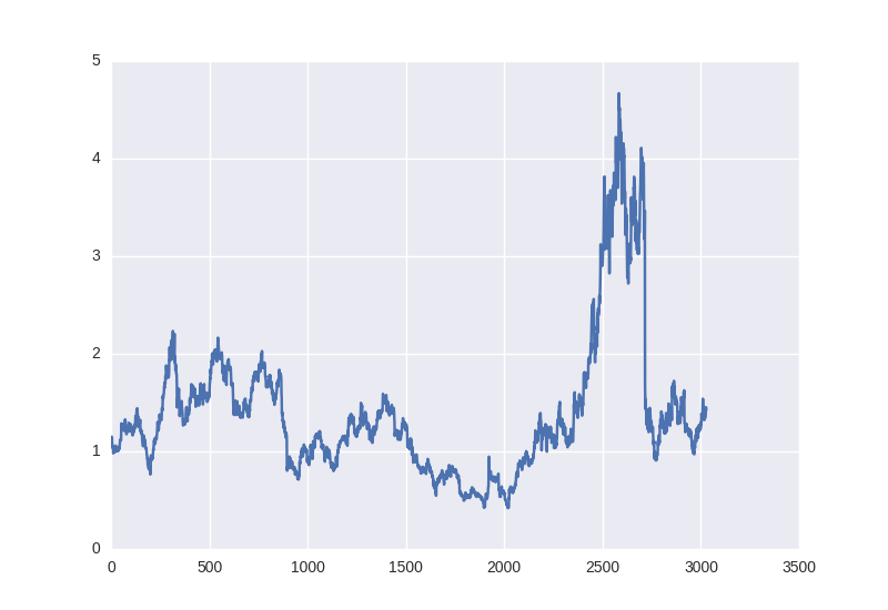
Figure 1

And in a friendly way, we cannot use the minimax or z-score normalization of these values according to our window, because if there are some characteristics within 30 days, they can also change the next day or in the middle of our window.

But if you look closely at the classification problem:

Dat = [(np.array(x) - np.mean(x)) / np.std(x) for x in Dat]

For the regression problem, this does not work because if we also subtract the average and divide by the deviation, we will have to restore this value for the price value the next day, and these parameters may be completely different.

Therefore, we will try two options:

Train the raw data and try to deceive the system by taking away the expectation or variance of the next day that is less interesting. We are only interested in moving up or down. Therefore, we will take risks and use z-scores to standardize our 30 day window, but they are limited to them and will not affect anything in the future:

Percentage change in price the next day - pandas will help us solve this problem:

close_price_diffs = close.price.pct_change()

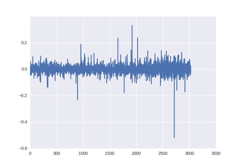
It looks like this. As we can see, these data are obtained without any operation with statistical characteristics and are already within the limit of - 0.5 to 0.5:

The training samples are divided. The first 85% of the time window is used for training and the last 15% is used to check the operation of the neural network.

Therefore, in order to train our neural network, we will receive the following X and Y pairs:

30 day closing price and [1,0] or [0,1], depending on the increase or decrease of the price value classification of the binary file; 30 day price percentage change and the second day change of regression.

Neural network architecture

We will use multilayer perceptron as the basic model. Let's take Keras as as an implementation framework - it's very simple and intuitive. You can use it to implement quite complex calculation diagrams, but we don't need it so far.

A basic grid is realized by 30 neurons and 64 neurons in the input layer (the first hidden layer), and then batch normalization - it is recommended to use it in almost all multilayer networks, and then the activation function (ReLU) has been considered abnormal, so let's take some fashionable functions like leaky relu.

At the output, we place a neuron (or two for classification). According to the task (classification or regression), it either has a softmax at the output or has no nonlinearity so that it can predict any value.

The classification codes are as follows:

model = Sequential()
model.add(Dense(64, input_dim=30))
model.add(BatchNormalization())
model.add(LeakyReLU())
model.add(Dense(2))
model.add(Activation('softmax'))

For regression problems, the activation parameter should finally be "linear".

Next, we need to define the error function and optimization algorithm. Without further discussing the details of gradient descent change, let's take Adam with step size of 0.001 as an example; the loss parameter of classification needs to be set as cross entropy -'categorical_crossentropy ', and the loss parameter of regression needs to be set as mean square error -'mse'.

Keras also allows us to control the training process very flexibly. For example, if our results do not improve, it is best to reduce the value of the gradient descent step - which is what reduce LR on platform does, and we add it as a callback to the model training.

reduce_lr = ReduceLROnPlateau(monitor='val_loss', factor=0.9, patience=5, min_lr=0.000001, verbose=1)
model.compile(optimizer=opt, 
              loss='categorical_crossentropy',
              metrics=['accuracy'])
Neural network training
history = model.fit(X_train, Y_train, 
          nb_epoch = 50, 
          batch_size = 128, 
          verbose=1, 
          validation_data=(X_test, Y_test),
          shuffle=True,
          callbacks=[reduce_lr])

After the learning process is completed, it is best to display a dynamic chart of error and accuracy values on the screen:

plt.figure()
plt.plot(history.history['loss'])
plt.plot(history.history['val_loss'])
plt.title('model loss')
plt.ylabel('loss')
plt.xlabel('epoch')
plt.legend(['train', 'test'], loc='best')
plt.show()
plt.figure()
plt.plot(history.history['acc'])
plt.plot(history.history['val_acc'])
plt.title('model accuracy')
plt.ylabel('acc')
plt.xlabel('epoch')
plt.legend(['train', 'test'], loc='best')
plt.show()

Before starting the training, I would like to draw your attention to an important point: it is necessary to learn a longer algorithm on such data, at least 50-100 epoch s.

This is because if you train 5-10 epochs and see 55% accuracy, it probably does not mean that you have learned to find patterns when analyzing training data. You will see that only 55% of the window is used for one mode (e.g. increase) and the remaining 45% is used for another mode (decrease).

In our example, 53% of the windows belong to the "decrease" category and 47% belong to the "increase" category, so we will try to obtain an accuracy higher than 53%, which shows that we have learned to find symbols.

When preparing training samples, the accuracy of original data (such as closing price and simple algorithm) is too high, which may indicate that the model is over fitted.

Forecasting financial time series - classification problem

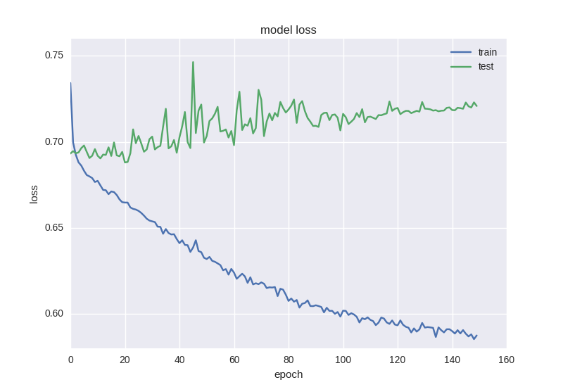
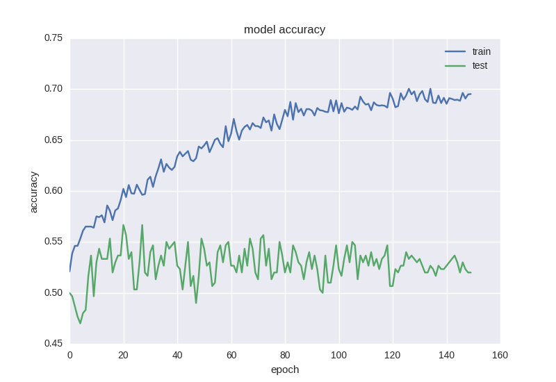
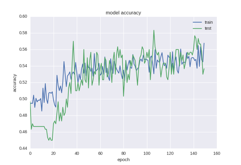
Let's train our first model and look at the chart:

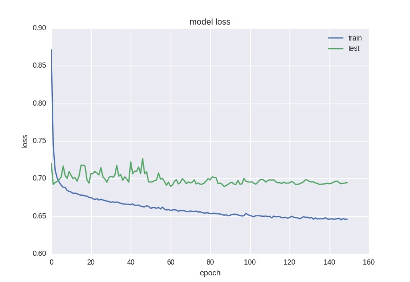
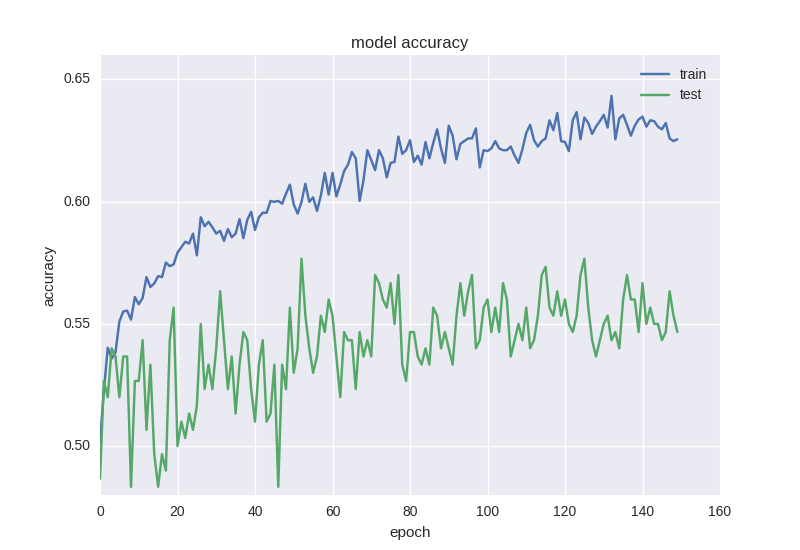
It can be seen that the accuracy of the test sample has been maintained at the error of ± 1 value, the error of the training sample has decreased, and the accuracy has increased, indicating that it has been fitted.

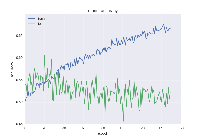
Let's look at a deeper two-tier model:

model = Sequential()

model.add(Dense(64, input_dim=30))

model.add(BatchNormalization())

model.add(LeakyReLU())

model.add(Dense(16))

model.add(BatchNormalization())

model.add(LeakyReLU())

model.add(Dense(2))

model.add(Activation('softmax'))

The following are the results of its work:

Roughly the same picture. When we face over fitting, we need to add regularization to our model.

In the process of regularization, we impose certain restrictions on the weight of the neural network so that there will be no large dispersion of the value. Although there are a large number of parameters (i.e. network weight), some of them are reversed and set to zero for simplicity.

We'll start with the most common way -- adding an additional term to the error function in the L2 norm of the sum of weights. In Keras, this is using Keras. Regulators. Activity_ The regularizer completes.

model = Sequential()
model.add(Dense(64, input_dim=30,
                activity_regularizer=regularizers.l2(0.01)))
model.add(BatchNormalization())
model.add(LeakyReLU())
model.add(Dense(16,
                activity_regularizer=regularizers.l2(0.01)))
model.add(BatchNormalization())
model.add(LeakyReLU())
model.add(Dense(2))
model.add(Activation('softmax'))

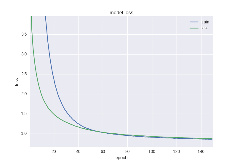
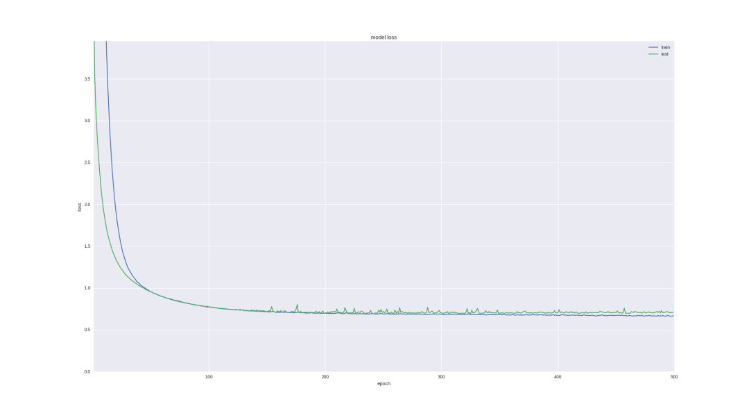
This neural network learns better in terms of error function, but its accuracy is still affected:

When processing data with a large number of noise or random properties, we often encounter strange effects such as error reduction rather than accuracy reduction - this is because the error is calculated based on cross entropy, which may be reduced, and accuracy is an indicator of neural elements with correct answers, which may remain incorrect even if the error changes.

Therefore, it is worth using the popular Dropout technology in recent years to add more regularization to our model - roughly speaking, this is to randomly "ignore" some weights in the learning process to avoid the common adaptation of neurons (so that they do not learn the same function). The code is as follows:

model = Sequential()
model.add(Dense(64, input_dim=30,
                activity_regularizer=regularizers.l2(0.01)))
model.add(BatchNormalization())
model.add(LeakyReLU())
model.add(Dropout(0.5))
model.add(Dense(16,
                activity_regularizer=regularizers.l2(0.01)))
model.add(BatchNormalization())
model.add(LeakyReLU())
model.add(Dense(2))
model.add(Activation('softmax'))

As you can see, we will "discard" the connection between the two hidden layers for each weight with a 50% probability during training. dropout is usually not added between the input layer and the first hidden layer, because in this case, we will learn from simple noise data, and it will not be added before output. Of course, there will be no drop during the network test. How can such a grid learn:

If you stop training the network earlier, we can get 58% accuracy in predicting price changes, which is certainly better than random guess.

Another interesting and intuitive moment in predicting the financial time series is that the volatility of the next day is random, but when we look at the chart and candle chart, we can still notice the trend in the next 5-10 days.

Let's check whether our neurons can handle such a task - we will use the last successful architecture to predict the price trend in five days, and we will train more epoch s:

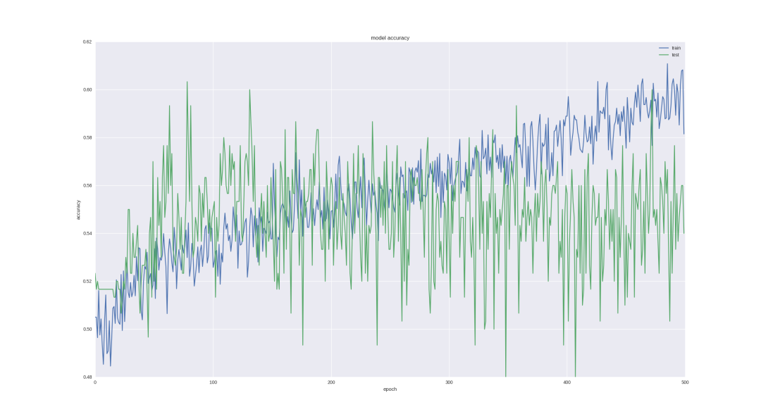
As you can see, if we stop training early enough (overtime, there will still be over fitting), then we can get 60% accuracy, which is very good.

Forecasting Financial Time Series -- regression problem

For the regression problem, let's adopt our last successful classification architecture (which has shown that it can learn the necessary features), remove Dropout, and conduct more iterative training.

In addition, in this case, we can not only view the error value, but also intuitively evaluate the prediction quality using the following code:

pred = model.predict(np.array(X_test))
original = Y_test
predicted = pred
plt.plot(original, color='black', label = 'Original data')
plt.plot(predicted, color='blue', label = 'Predicted data')
plt.legend(loc='best')
plt.title('Actual and predicted')
plt.show()
The network architecture will look like this:
model = Sequential()
model.add(Dense(64, input_dim=30,
                activity_regularizer=regularizers.l2(0.01)))
model.add(BatchNormalization())
model.add(LeakyReLU())
model.add(Dense(16,
                activity_regularizer=regularizers.l2(0.01)))
model.add(BatchNormalization())
model.add(LeakyReLU())
model.add(Dense(1))
model.add(Activation('linear'))

Let's see what happens if we train on the "original" adjusted closing price:

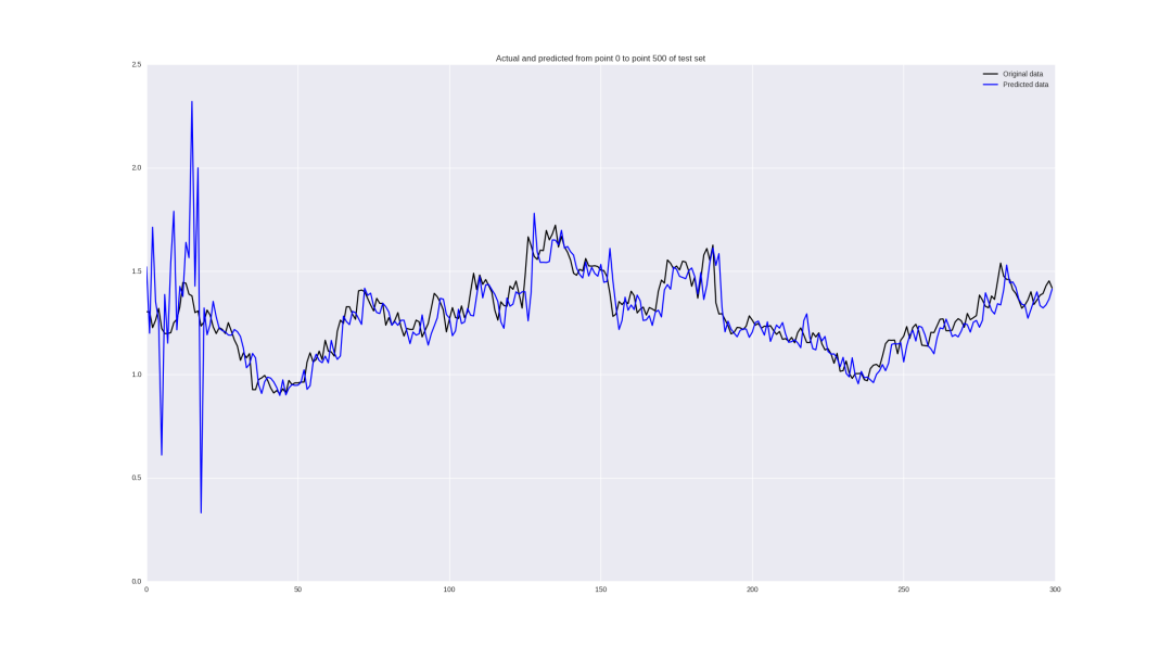
It looks good from a distance, but if we look carefully, we will find that our neural network is only backward in its prediction, which can be regarded as failure.

For price changes, the result is:

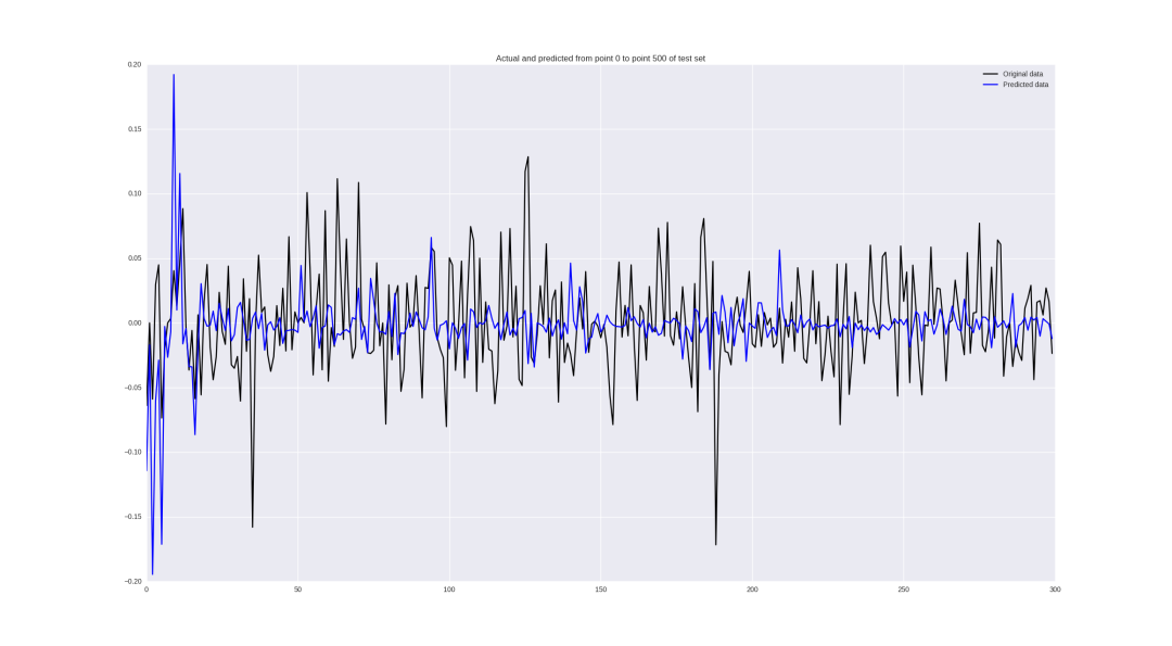
Some values are predicted well, some local trends are guessed correctly, but in general - sloppy.

discuss

In principle, the results are usually not impressive at first glance. It is true, but we train the simplest neural network on one-dimensional data without much preprocessing. There are many steps to improve your accuracy to 60-70%:

• Use not only the closing price, but also all the data in our. csv (highest price, lowest price, opening price, closing price, trading volume) - that is, pay attention to all the information available at any given time
• Optimize the super parameters - window size, number of neurons in the hidden layer, training steps - all these parameters are taken randomly. Using random search, you can find that maybe we need to look at the deeper grid 45 days ago and learn in smaller steps.
• Use a loss function that is more suitable for our task (for example, in order to predict price changes, we can find a neural function with incorrect symbols, and the symbol of the usual MSE to the number is unchanged)

conclusion

In this paper, we apply the simplest neural network architecture to predict the price trend of the market. This pipeline can be used for any time series, mainly to select the correct data preprocessing, determine the network architecture, and evaluate the quality of the algorithm.

In our example, we managed to use the price window of the first 30 days to predict the trend of 5 days with 60% accuracy, which can be considered as a good result. The quantitative prediction results of price changes proved to be failed. For this task, it is recommended to use more serious tools and statistical analysis of time series.