Drawing with Fourier series
click Go to view the effect
theoretical basis
Fourier series:
Those who have learned Fourier series, Fourier transform and other knowledge know that the [periodic function] satisfying the [Dirichlet condition] can be fitted with Fourier series.
Dirichlet condition:
- x(t) shall be absolutely integrable in any cycle; In any finite interval, x(t) can only take finite maximum or minimum values;
- On any finite interval, x(t) can only have finite numbers Type I discontinuity.
Fourier series expression:
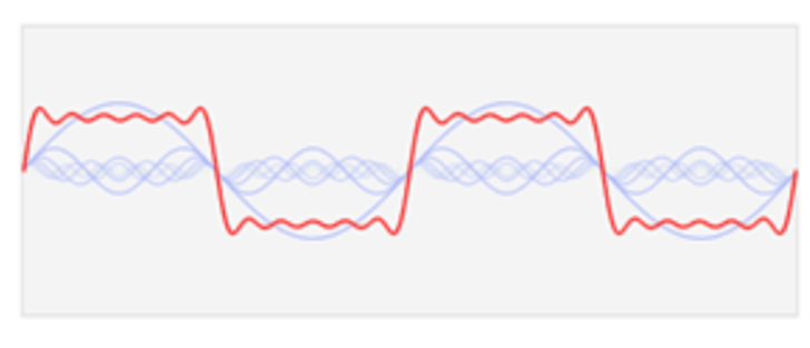
So, another way of thinking, can we also use Fourier series to draw all kinds of lines and combine them into all kinds of graphics? The answer is yes
Principle understanding
Transformation between plane point and f(t)
Two dimensional images are composed of some points. The position of the point is determined by the (x, y) coordinates [take the xy plane as an example], so the coordinates of a point can be represented by a complex number:
f(t) can be complex. Adding a series of points can get f(t) at a certain time, so it can be expanded by Fourier series.
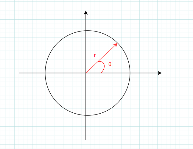
Relationship between complex number and circle
Students who have studied complex variable functions know that a complex number can be converted as follows:
Therefore:
The complex number can represent either a point or a vector, so r can be expressed as the length of the vector, θ Can be expressed as the angle of the vector, when θ When it changes within the range of $[0,2 \ PI] $, it means that the vector is rotating around the origin to form a circle.
Get back to the point
Look at this equation again:
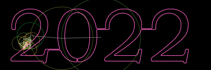
f(t) represents a point of the graph we want to draw at time t, and the complex index \ (a_ke^{jk\omega t} \) on the right represents that at a certain time t, the vector length is \ (a_k \) and the angle is \ (jk\omega t \), ω That is, the rotation speed of the vector.
Therefore, the right side represents the addition of countless vectors. With the continuous increase of time t and the continuous rotation of vectors, we can continuously calculate all points represented by \ (f(t) \), and connect these points to form the graph we want.
Note: it is necessary to ensure that a figure can be drawn in one stroke, that is, a simply connected figure, such as a square;
Multiple graphs can use \ (f_1(t) and f respectively_ 2(t),f_3(t) \) and so on.
The (x, y) coordinates of a graph are determined by us in advance, that is, we have to determine what graph we want to draw in advance, and then extract the (x, y) coordinates of its contour. Later, we will introduce how to extract the image contour through python
If you determine the (x,y) coordinates, that is, you determine f(t), because f(t) can be a complex number
Now we mainly solve how to expand \ (f(t) \) into Fourier series, that is, determine
-
t is a time scale, which changes with time and does not need us to find it;
-
T is the period of f(t), which is determined by the graph we draw, that is, how often we draw the graph, usually the number of points of the graph (outline).
The unit of T should be seconds. Why is it points? In fact, all points N of the contour are used to represent the number of points drawn in a cycle, so that the graph is drawn just once;
-
j is understood to mean that this is a plural, regardless;
-
\(a_k \) is the only parameter we require, that is, the length value of each vector;
When learning Fourier series, we all know that the coefficient \ (a_k \) is solved as follows:
This is an expression under the condition that t is continuous. We can turn it into a discrete case (t changes to \ (\ Delta t \) each time):
The next step is how to calculate \ (a_k \) through code
Note that the range of K \ (k =... - 2, - 1,0,1,2... \) k represents the number of circles. It is determined by yourself. The greater the K, the better the approximation effect. However, the greater the K, the higher the computational complexity and higher requirements for computer performance. It is recommended that the maximum number of points should not exceed N (i.e. all points of f(t))
After learning digital signal processing, you can see the formula of DFT
Where \ (X(k) \) is actually \ (a_k \), \ (x(n) \) is \ (f(t) \)
code implementation
Find the coefficients of Fourier series
Programming language Javascript
First realize the addition and multiplication of complex numbers, and convert the complex index into a general index
In the code, z=[a, b] is used to represent a complex number z=a+jb. In fact, the representation does not matter. As long as a complex number can be determined, it is important to enable it to realize some basic operations of complex numbers
//Complex multiplication
//z1 = a1 + jb1, denoted by [a1, b1]
//z2 = a2 + jb2, represented by [a2, b2]
function complexMul(z1, z2) {
    return [z1[0] * z2[0] - z1[1] * z2[1], z1[0] * z2[1] + z2[0] * z1[1]];
}

// Complex addition
function complexAdd(z1, z2) {
    return [z1[0] + z2[0], z1[1] + z2[1]];
}

// Complex exponential to complex, z=r*(e^j) θ)= r*cos( θ)+ r*jsin( θ)  among θ Is plural
function r_exp(r, theta) {
    return [r * Math.cos(theta), r * Math.sin(theta)];
}
Then find \ (a_k \), (represented by "Cn" in the code), and carefully figure out the formula when writing:
// K=[0, -1,1, -2,2, -3,3 ...]
function get_K(circleCounts){
    var K = [];  //length = circleCount
    for (var i = 0; i < circleCounts; i++) {
        K[i] = (1 + i >> 1) * (i & 1 ? -1 : 1); //K = [0, -1,1, -2,2, -3,3, -4,4,...]
    }
    return K;
}
//Parameter xn, that is, the coordinate set of f(t),
//circleCounts: that is, the size of k
//L is not required for solving Fourier series. It is used to represent the magnification of Cn, that is, the magnification of vector length, which can enlarge the last drawn figure
function get_Cn(xn, circleCounts, L=1){
    xn_len = xn.length;
    Cn = []       //N is the number of circles
    K = get_K(circleCounts);
    for(var k=0; k<circleCounts; k++){
        Cn[k] = [0, 0];
        for(var n=0; n<xn_len;n++){
            Cn[k] = complexAdd(Cn[k], complexMul(xn[n], r_exp(1, -2*PI*K[k]*n/xn_len)));
        }
        Cn[k][0] /= (xn_len/L);
        Cn[k][1] /= (xn_len/L);
    }
    return Cn;
}
Find Fourier series
Then find \ (f(t) \) according to \ (a_k \), that is, add up the vectors
// CX and CY are used to determine where to draw the image, that is, positioning
// n, that is, circleCounts, the greater the approximation effect, the better, but it will also lead to higher performance consumption
// imgIndex indicates which image to draw, because you want to draw several images at the same time, such as f1(t), f2(t), f3(t)
// Speed is used to indicate the drawing speed
function DrawPath(cx, cy, n = 5, imgIndex=0, speed=1) {
    let p = [cx, cy];
    //Sum vectors
    for (var k = 0; k < n; k++) {
        var W = r_exp(1, 2 * PI * (time_n * speed) * K[k] / imgxn[imgIndex].length);   // W-factor
        p = complexAdd(p, complexMul([imgCn[imgIndex][k][0], imgCn[imgIndex][k][1]], W));
    }
    var x = p[0];
    var y = p[1];
    valuePointer[imgIndex] = valuePointer[imgIndex]+1;
    values_x[imgIndex][valuePointer[imgIndex] & pointCount[imgIndex]] = x;
    values_y[imgIndex][valuePointer[imgIndex] & pointCount[imgIndex]] = y;
    context.beginPath();
    context.lineWidth = 2
    context.strokeStyle = "rgba(255,100,200,1)";
    context.moveTo(x, y);
    for (var i = 1; i <= pointCount[imgIndex]; ++i) {
        context.lineTo(values_x[imgIndex][(valuePointer[imgIndex] - i) & pointCount[imgIndex]], values_y[imgIndex][(valuePointer[imgIndex] - i) & pointCount[imgIndex]]);
    }
    context.stroke();
}
Draw circles and vectors:
function DrawCircles(cx, cy, n = 5, imgIndex=0, speed=1) {
    let p = [cx, cy];  //Center of the first circle
    for (var k = 0; k < n; k++) {
        context.beginPath();
        var r = Math.hypot(imgCn[imgIndex][k][0], imgCn[imgIndex][k][1]);
        context.arc(p[0], p[1], r, 0, 2 * PI);
        context.lineWidth = 1;
        context.strokeStyle = "rgba(100,150,60,1.0)";
        if (k != 0) {
            context.stroke();   //The first circle is not drawn
        }
        var W = r_exp(1, 2 * PI * (time_n * speed) * K[k] / imgxn[imgIndex].length);   // W-factor
        p = complexAdd(p, complexMul([imgCn[imgIndex][k][0], imgCn[imgIndex][k][1]], W));
    }
}
function DrawLines(cx, cy, n=5, imgIndex=0, speed=1) {
    context.beginPath();
    let p = [cx, cy];  //The center of the first circle, used to locate the entire drawing
    for (var k = 0; k < n; k++) {

        context.moveTo(p[0], p[1]); //The first line is not drawn
        var W = r_exp(1, 2 * PI * (time_n * speed) * K[k] / imgxn[imgIndex].length);   // W-factor
        p = complexAdd(p, complexMul(imgCn[imgIndex][k], W));
        if(k==0) continue;
        context.lineTo(p[0], p[1]);
    }
    context.lineWidth = 1;
    context.strokeStyle = "rgba(255,255,255,0.8)";
    // context.strokeStyle = "rgba(" + randomx(255) + "," + randomx(255) + "," + randomx(255) + ",0.5)";

    context.stroke();
}
How to extract image contour through python
These are the basic codes required for drawing graphics, but there is another important problem: how to obtain the outline of graphics, that is, obtain \ (f(t) \) [xn in the code]. Only by obtaining \ (f(t) \) first can we obtain \ (a_k \) [Cn in the code]
Method 1
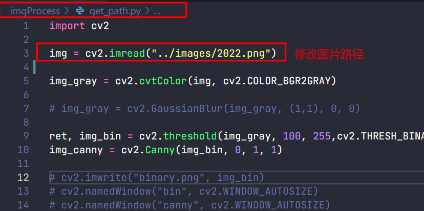
The image contour can be easily obtained through OpenCV. Python 3 calls the opencv library to extract the image contour:
import cv2
img = cv2.imread("../images/kuaile.png") #Read picture
img_gray = cv2.cvtColor(img, cv2.COLOR_BGR2GRAY) # Convert to grayscale
img_gray = cv2.GaussianBlur(img_gray, (1,1), 0, 0) # Gaussian blur
#Turn to binary graph, and those less than the threshold will turn to pure black
ret, img_bin = cv2.threshold(img_gray, 100, 255,cv2.THRESH_BINARY)
#Extract contour
img_canny = cv2.Canny(img_bin, 0, 1, 1)
cv2.imshow("bin", img_bin)
cv2.imshow("canny", img_canny)
_, contours, hierarchy = cv2.findContours(img_canny, cv2.RETR_EXTERNAL, cv2.CHAIN_APPROX_NONE)
cv2.drawContours(img, contours, -1, (255, 0, 255), 1) #The rightmost parameter is the line thickness
cv2.imshow("result", img)
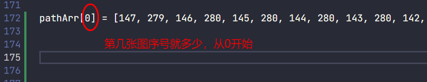
# Write contour xy coordinates to path Txt in the format pathArr[]=[x1, y1, x2, y2,...]
with open("./path.txt", 'w') as f:
f.write("pathArr[]=[")
for i in contours:
for j in i:
f.write(str(j[0][0]))
f.write(",")
f.write(str(j[0][1]))
f.write(",")
f.write("];")
cv2.waitKey(5000)
cv2.destroyAllWindows()
This is the generated path Txt

Method 2
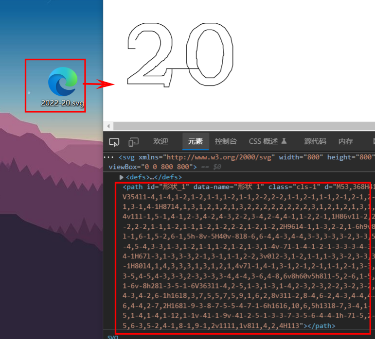
If you are familiar with svg, you can make it into svg vector graph (draw the outline of the graph you need to draw through tools such as photoshop, and then save it as svg picture), or you can extract path
import numpy as np
from svg.path import parse_path

path = """
M53,368H41V354l1-4,1-4,1-2,1-2,1-1,1-2,1-1,2-2,2-2,1-1,2-1,1-1,2-1,2-1,2-1,3-1,4-1H87l4,1,3,1,2,1,2,1,3,2,2,2,2,2,2,2,2,3,1,2,1,2,1,3,1,4v11l-1,5-1,4-1,2-3,4-2,4-3,2-2,3-4,2-4,4-1,1-2,2-1,1H86v1l-2,2-2,2-2,1-1,1-2,1-1,1-2,1-2,2-2,1-2,1-2,2H96l4-1,1-3,2-2,1-6h9v8l-1,6-1,5-2,6-1,5h-8v-5H40v-8l8-6,6-4,4-3,4-4,3-3,3-3,3-2,3-3,5-4,5-4,3-3,1-3,1-2,1-1,1-2,1-2,1-3,1-4v-7l-1-4-1-2-1-3-3-3-4-3-4-1H67l-3,1-3,3-3,2-1,3-1,1-1,2-2,3v0l2-3,1-2,1-1,1-3,3-2,3-3,3-1H80l4,1,4,3,3,3,1,3,1,2,1,4v7l-1,4-1,3-1,2-1,2-1,1-1,2-1,3-3,3-5,4-5,4-3,3-3,2-3,3-3,3-4,4-4,3-6,4-8,6v8h60v5h8l1-5,2-6,1-5,1-6v-8h28l-3-5-1-6V363l1-4,2-5,1-3,1-3,1-4,2-3,2-3,2-2,3-2,3-2,4-3,4-2,6-1h16l8,3,7,5,5,7,5,9,1,6,2,8v31l-2,8-4,6-2,4-3,4-4,4-6,4-4,2-7,2H168l-9-3-8-7-5-5-4-7-1-6h16l6,10,6,5h13l8-7,3-4,1-5,1-4,1-4,1-12,1-1v-4l-1-9v-4l-2-5-1-3-3-7-3-5-6-4-4-1h-7l-5,2-5,6-3,5-2,4-1,8-1,9-1,2v11l1,1v8l1,4,2,4H113
"""

ps = parse_path(path)
xy = []
for p in ps:
    if p.length() == 0:
        continue
    xy.append([p.start.real, p.start.imag])


with open("./path.txt", 'w') as f:
    f.write("pathArr[]=[")
    for i in xy:
        f.write(str(int(i[0])))
        f.write(",")
        f.write(str(int(i[1])))
        f.write(",")
    f.write("];")
The two methods have their own advantages and disadvantages, which can be selected according to their familiarity
Code usage
The complete code has been put into Git Code and Gitee of CSDN. If you need to use it, go to download it yourself
Note: Method 1 is used to obtain the path, and method 2 is similar to that of method 1
-
First, prepare a picture (the outline of the picture can be drawn in one stroke, preferably black and white and obvious), such as:

-
Modify imgProcess/get_path.py picture path
-
Open imgprocess / path Txt, copy all the data (there will be more) to myft / JS / main JS is located as follows
-
initialization
//The parameters are:
//The first pathArr, here is 0
//The number of circles (400 by default). Select 500 here
//The path storage capacity (11 by default, 2 * * 11 after internal calculation) is not modified here
//Magnification (default 1), no magnification here
initImg(0, 500, 11, 1);
-
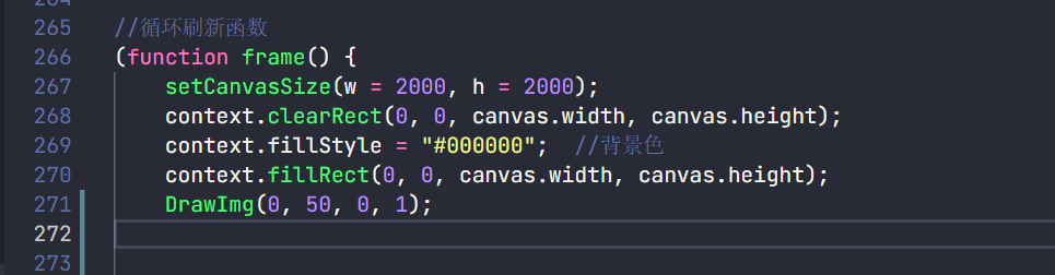
mapping
Call the DrawImg function, and the parameters are [x coordinate (0), y coordinate (50), the drawing number (0 here), and drawing speed (1 here)]
Note: the xy coordinate here is only the approximate position
-
After modification, open myft / index HTML to view the effect
Reference tutorial Coding Abas - teach you how to write Fourier animation (the author's writing is very good. I just read what he wrote and understood it. Then I copied it myself. I can learn from it.)