feature selection

Reason for feature selection

• Redundancy: some features have high correlation and are easy to consume computing performance

• Noise: some features have a negative impact on the prediction results

What is feature selection

Feature selection is simply to select some features from all the extracted features as the features of the training set,
The value of features can be changed or not changed before and after selection, but the dimension of features after selection is different
It's smaller than before. After all, we only selected some of the features.

Main methods (three weapons):

• Filter: VarianceThreshold

• Embedded: regularization, decision tree

• Wrapper (wrapped)

VarianceThreshold method API:

sklearn.feature_selection.VarianceThreshold

VarianceThreshold syntax

• VarianceThreshold(threshold = 0.0):
  Delete all low variance features

• Variance.fit_transform(X,y):
  10: Data in numpy array format [n_samples,n_features];
  Return value: features whose training set difference is lower than threshold will be deleted;
  The default value is to retain all non-zero variance features, that is, delete features with the same value in all samples.

VarianceThreshold process

1. Initialize VarianceThreshold and specify the threshold as difference
2. Call fit_transform

[[0, 2, 0, 3],
[0, 1, 4, 3],
[0, 1, 1, 3]]

Example:

from sklearn.feature_selection import VarianceThreshold

def var():
    """
    feature selection -Delete features with low variance
    :return: None
    """
    var = VarianceThreshold(threshold=0.0)

    data = var.fit_transform([[0, 2, 0, 3], [0, 1, 4, 3], [0, 1, 1, 3]])

    print(data)
    return None

if __name__ == "__main__":
    var()

Operation results:
The column with variance of 0 is removed

[[2 0]
 [1 4]
 [1 1]]

Other feature selection methods: neural network

sklearn dimension reduction principal component analysis

API:

sklearn. decomposition

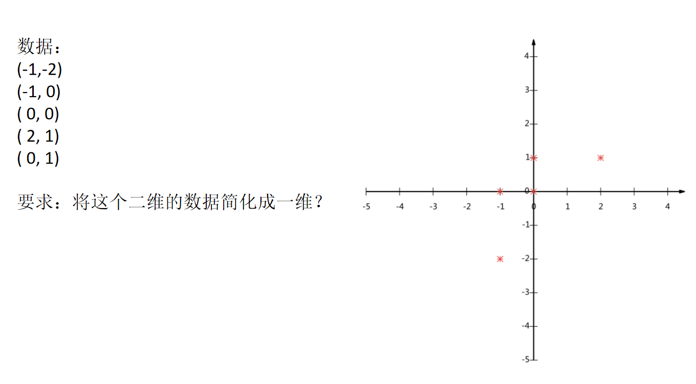
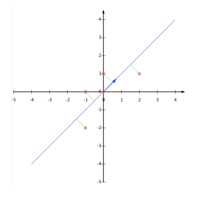
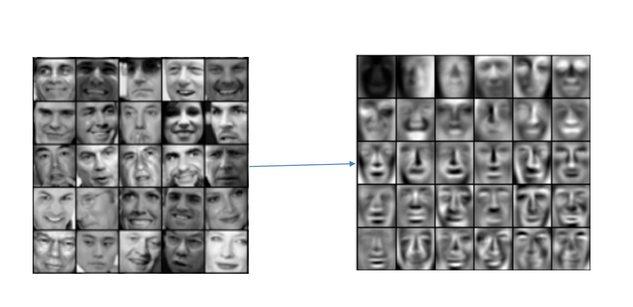
PCA (principal component analysis)

PCA is a technique for analyzing and simplifying data sets.

The purpose is to reduce the dimension (complexity) of the original data and lose a small amount of information.

Function: it can reduce the number of features in regression analysis or cluster analysis

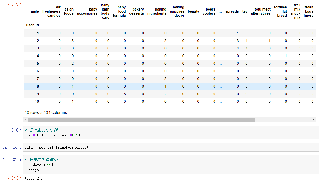
PCA syntax

• PCA(n_components=None):
  Decompose the data into lower dimensional space;
  n_components is decimal, indicating the percentage information to be retained, such as 0.9 → 90%;
  n_components is an integer indicating the number of features reduced. It is generally not used.

• PCA.fit_transform(X):
  10: Data in numpy array format [n_samples,n_features]
  Return value: array of the specified dimension after conversion

PCA process

1. Initialize PCA and specify the reduced dimension
2. Call fit_transform

[[2,8,4,5],
[6,3,0,8],
[5,4,9,1]]

Example:

from sklearn.decomposition import PCA

def pca():
    """
    Principal component analysis for feature dimensionality reduction
    :return: None
    """
    pca = PCA(n_components=0.9)

    data = pca.fit_transform([[2,8,4,5],[6,3,0,8],[5,4,9,1]])

    print(data)

    return None

if __name__ == "__main__":
    pca()

Operation results:

[[ 0.          3.82970843]
 [-5.74456265 -1.91485422]
 [ 5.74456265 -1.91485422]]

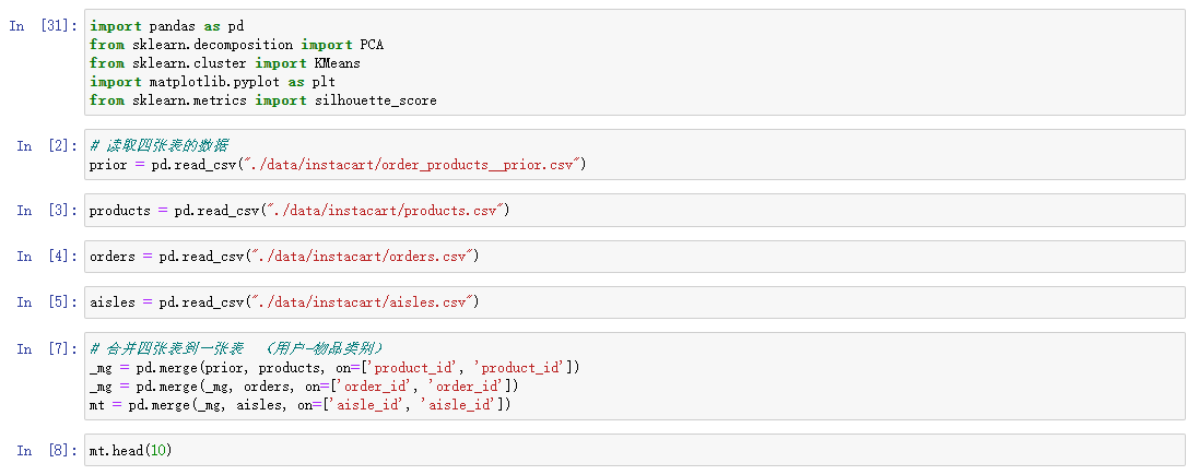
Dimensionality reduction case

The dimension reduction is subdivided according to the user's preference for the item category.

Data:

• products.csv: product information
• order_ products__ Priority.csv: order and item information
• orders.csv: user's order information
• aisles.csv: the specific item category to which the commodity belongs

Because users and item categories are not in the same table, it is necessary to merge table information according to the same characteristics of different tables.

1. Merge all tables into one table

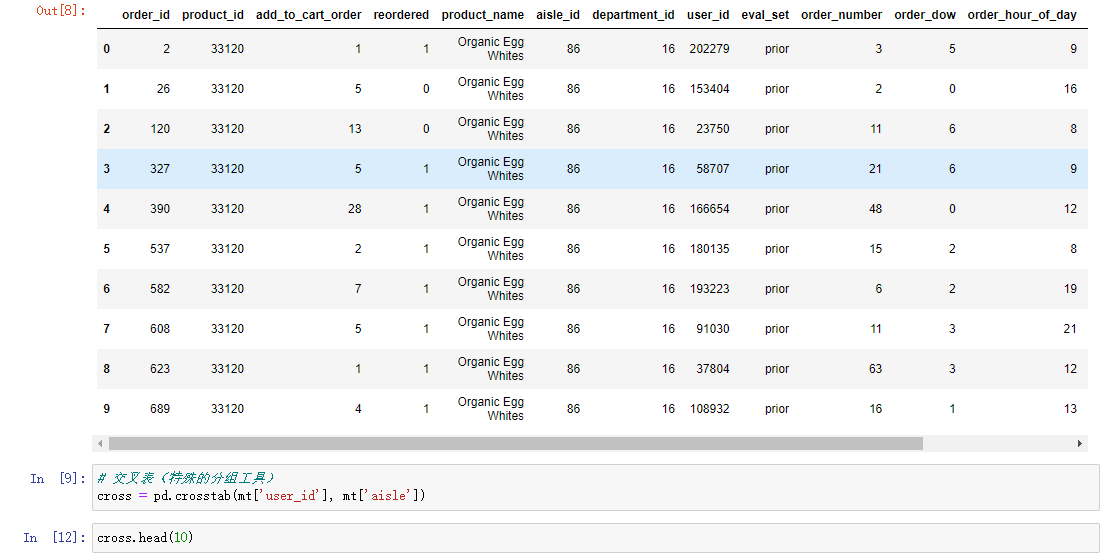
2. Create a similar row and column data

Crosstab (special grouping table)

3. Principal component analysis

Other dimensionality reduction methods

Linear discriminant analysis LDA

Fundamentals of machine learning

1. Machine learning development process

2. What is the machine learning model

3. Classification of machine learning algorithms

Algorithm is the core, data and calculation are the foundation

Classification of machine learning algorithms

• Supervised learning (prediction)

Classification (the target value is discrete): k-nearest neighbor algorithm, Bayesian classification, decision tree and random forest, logical regression, neural network

Regression (the target value is continuous): linear regression and ridge regression

Annotated hidden Markov model (not required)

• Unsupervised learning
  Clustering k-means

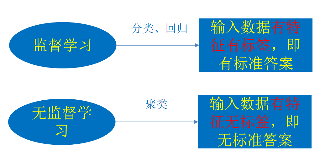
Supervised learning

Supervised learning (English: supervised learning) can be learned from input data
To or build a model and infer new results according to this model. The input data is generated by
The input consists of eigenvalues and target values. The output of a function can be a continuous value
(called regression), or the output is a finite number of discrete values (called classification).

Unsupervised learning

Unsupervised learning (English: Supervised learning) can be obtained from the input data
Learn or build a model and infer new results according to this model. The input data is
It consists of input eigenvalues.

classification problem

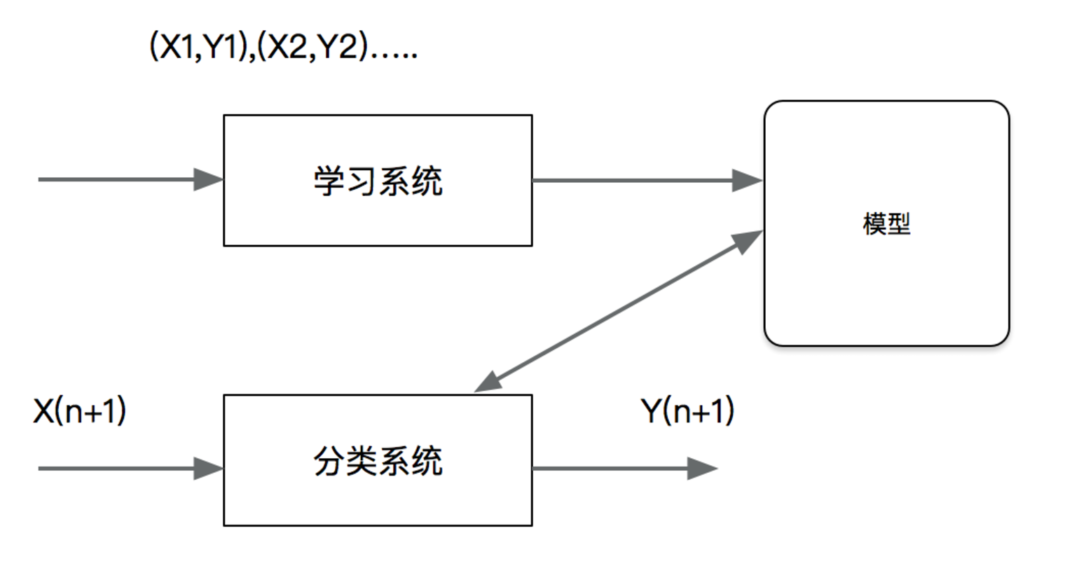
Concept: classification is a core problem of supervised learning. In supervised learning, when the output variables take finite discrete values, the prediction problem becomes a classification problem. The most basic is the binary classification problem, that is, judge right and wrong, and select one of the two categories as the prediction result.

Application of classification problems:

Classification is to "classify" data according to its characteristics, so it is widely used in many fields

In banking business, build a customer classification model to classify customers according to the size of loan risk

In image processing, classification can be used to detect whether there are faces, animal categories and so on in the image

In handwriting recognition, classification can be used to recognize handwritten numbers

Text classification, where the text can be news reports, web pages, e-mail, academic papers

Regression problem

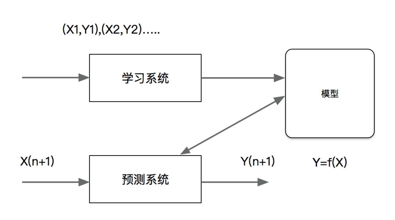
Concept: regression is another important issue in supervised learning. Regression is used to predict the relationship between input variables and output variables, and the output is a continuous value.

Application of regression problem:

Regression is also widely used in many fields

House price forecast: make a forecast according to the historical house price data of a place

Financial information, daily stock trend

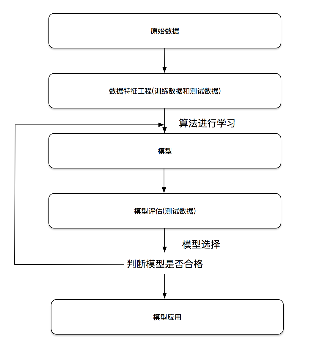
Machine learning development process

sklearn dataset

1. Data set partition
2. Introduction to sklearn dataset interface
3. sklearn classification dataset
4. sklearn regression dataset

Data set partition

The general data set of machine learning is divided into two parts:

Training data: used for training and building models

Test data: used in model verification to evaluate whether the model is effective

sklearn dataset partitioning API:

sklearn.model_selection.train_test_split

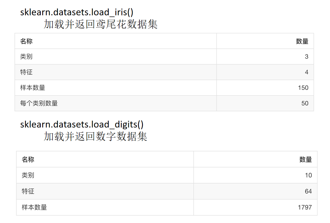
Introduction to scikit learn dataset API

• sklearn.datasets
  Load get popular dataset

• datasets.load_*()
  Obtain small-scale data sets, and the data is contained in datasets

• datasets.fetch_*(data_home=None)
  To obtain large-scale data sets, you need to download them from the network. The first parameter of the function is data_home indicates the directory where the dataset is downloaded. The default is ~ / scikit_learn_data/

Gets the type returned by the dataset

Data type returned by load and fetch datasets.base.bunch (dictionary format)

Data: feature data array, which is a two-dimensional numpy.ndarray array of [n_samples * n_features]

target: tag array, n_ One dimensional numpy.ndarray array of samples

Desc: Data Description

feature_names: feature name, news data, handwritten digits, regression data set

target_names: tag name. The regression data set has no

Example:

from sklearn.datasets import load_iris

li = load_iris()

print("Get eigenvalue")
print(li.data)
print("target value")
print(li.target)
print(li.DESCR)

Operation results:

Get eigenvalue
[[5.1 3.5 1.4 0.2]
 [4.9 3.  1.4 0.2]
 [4.7 3.2 1.3 0.2]
 [4.6 3.1 1.5 0.2]
 [5.  3.6 1.4 0.2]
 [5.4 3.9 1.7 0.4]
 [4.6 3.4 1.4 0.3]
 [5.  3.4 1.5 0.2]
 [4.4 2.9 1.4 0.2]
 [4.9 3.1 1.5 0.1]
 [5.4 3.7 1.5 0.2]
 [4.8 3.4 1.6 0.2]
 [4.8 3.  1.4 0.1]
 [4.3 3.  1.1 0.1]
 [5.8 4.  1.2 0.2]
 [5.7 4.4 1.5 0.4]
 [5.4 3.9 1.3 0.4]
 [5.1 3.5 1.4 0.3]
 [5.7 3.8 1.7 0.3]
 [5.1 3.8 1.5 0.3]
 [5.4 3.4 1.7 0.2]
 [5.1 3.7 1.5 0.4]
 [4.6 3.6 1.  0.2]
 [5.1 3.3 1.7 0.5]
 [4.8 3.4 1.9 0.2]
 [5.  3.  1.6 0.2]
 [5.  3.4 1.6 0.4]
 [5.2 3.5 1.5 0.2]
 [5.2 3.4 1.4 0.2]
 [4.7 3.2 1.6 0.2]
 [4.8 3.1 1.6 0.2]
 [5.4 3.4 1.5 0.4]
 [5.2 4.1 1.5 0.1]
 [5.5 4.2 1.4 0.2]
 [4.9 3.1 1.5 0.2]
 [5.  3.2 1.2 0.2]
 [5.5 3.5 1.3 0.2]
 [4.9 3.6 1.4 0.1]
 [4.4 3.  1.3 0.2]
 [5.1 3.4 1.5 0.2]
 [5.  3.5 1.3 0.3]
 [4.5 2.3 1.3 0.3]
 [4.4 3.2 1.3 0.2]
 [5.  3.5 1.6 0.6]
 [5.1 3.8 1.9 0.4]
 [4.8 3.  1.4 0.3]
 [5.1 3.8 1.6 0.2]
 [4.6 3.2 1.4 0.2]
 [5.3 3.7 1.5 0.2]
 [5.  3.3 1.4 0.2]
 [7.  3.2 4.7 1.4]
 [6.4 3.2 4.5 1.5]
 [6.9 3.1 4.9 1.5]
 [5.5 2.3 4.  1.3]
 [6.5 2.8 4.6 1.5]
 [5.7 2.8 4.5 1.3]
 [6.3 3.3 4.7 1.6]
 [4.9 2.4 3.3 1. ]
 [6.6 2.9 4.6 1.3]
 [5.2 2.7 3.9 1.4]
 [5.  2.  3.5 1. ]
 [5.9 3.  4.2 1.5]
 [6.  2.2 4.  1. ]
 [6.1 2.9 4.7 1.4]
 [5.6 2.9 3.6 1.3]
 [6.7 3.1 4.4 1.4]
 [5.6 3.  4.5 1.5]
 [5.8 2.7 4.1 1. ]
 [6.2 2.2 4.5 1.5]
 [5.6 2.5 3.9 1.1]
 [5.9 3.2 4.8 1.8]
 [6.1 2.8 4.  1.3]
 [6.3 2.5 4.9 1.5]
 [6.1 2.8 4.7 1.2]
 [6.4 2.9 4.3 1.3]
 [6.6 3.  4.4 1.4]
 [6.8 2.8 4.8 1.4]
 [6.7 3.  5.  1.7]
 [6.  2.9 4.5 1.5]
 [5.7 2.6 3.5 1. ]
 [5.5 2.4 3.8 1.1]
 [5.5 2.4 3.7 1. ]
 [5.8 2.7 3.9 1.2]
 [6.  2.7 5.1 1.6]
 [5.4 3.  4.5 1.5]
 [6.  3.4 4.5 1.6]
 [6.7 3.1 4.7 1.5]
 [6.3 2.3 4.4 1.3]
 [5.6 3.  4.1 1.3]
 [5.5 2.5 4.  1.3]
 [5.5 2.6 4.4 1.2]
 [6.1 3.  4.6 1.4]
 [5.8 2.6 4.  1.2]
 [5.  2.3 3.3 1. ]
 [5.6 2.7 4.2 1.3]
 [5.7 3.  4.2 1.2]
 [5.7 2.9 4.2 1.3]
 [6.2 2.9 4.3 1.3]
 [5.1 2.5 3.  1.1]
 [5.7 2.8 4.1 1.3]
 [6.3 3.3 6.  2.5]
 [5.8 2.7 5.1 1.9]
 [7.1 3.  5.9 2.1]
 [6.3 2.9 5.6 1.8]
 [6.5 3.  5.8 2.2]
 [7.6 3.  6.6 2.1]
 [4.9 2.5 4.5 1.7]
 [7.3 2.9 6.3 1.8]
 [6.7 2.5 5.8 1.8]
 [7.2 3.6 6.1 2.5]
 [6.5 3.2 5.1 2. ]
 [6.4 2.7 5.3 1.9]
 [6.8 3.  5.5 2.1]
 [5.7 2.5 5.  2. ]
 [5.8 2.8 5.1 2.4]
 [6.4 3.2 5.3 2.3]
 [6.5 3.  5.5 1.8]
 [7.7 3.8 6.7 2.2]
 [7.7 2.6 6.9 2.3]
 [6.  2.2 5.  1.5]
 [6.9 3.2 5.7 2.3]
 [5.6 2.8 4.9 2. ]
 [7.7 2.8 6.7 2. ]
 [6.3 2.7 4.9 1.8]
 [6.7 3.3 5.7 2.1]
 [7.2 3.2 6.  1.8]
 [6.2 2.8 4.8 1.8]
 [6.1 3.  4.9 1.8]
 [6.4 2.8 5.6 2.1]
 [7.2 3.  5.8 1.6]
 [7.4 2.8 6.1 1.9]
 [7.9 3.8 6.4 2. ]
 [6.4 2.8 5.6 2.2]
 [6.3 2.8 5.1 1.5]
 [6.1 2.6 5.6 1.4]
 [7.7 3.  6.1 2.3]
 [6.3 3.4 5.6 2.4]
 [6.4 3.1 5.5 1.8]
 [6.  3.  4.8 1.8]
 [6.9 3.1 5.4 2.1]
 [6.7 3.1 5.6 2.4]
 [6.9 3.1 5.1 2.3]
 [5.8 2.7 5.1 1.9]
 [6.8 3.2 5.9 2.3]
 [6.7 3.3 5.7 2.5]
 [6.7 3.  5.2 2.3]
 [6.3 2.5 5.  1.9]
 [6.5 3.  5.2 2. ]
 [6.2 3.4 5.4 2.3]
 [5.9 3.  5.1 1.8]]
target value
[0 0 0 0 0 0 0 0 0 0 0 0 0 0 0 0 0 0 0 0 0 0 0 0 0 0 0 0 0 0 0 0 0 0 0 0 0
 0 0 0 0 0 0 0 0 0 0 0 0 0 1 1 1 1 1 1 1 1 1 1 1 1 1 1 1 1 1 1 1 1 1 1 1 1
 1 1 1 1 1 1 1 1 1 1 1 1 1 1 1 1 1 1 1 1 1 1 1 1 1 1 2 2 2 2 2 2 2 2 2 2 2
 2 2 2 2 2 2 2 2 2 2 2 2 2 2 2 2 2 2 2 2 2 2 2 2 2 2 2 2 2 2 2 2 2 2 2 2 2
 2 2]
.. _iris_dataset:

Iris plants dataset
--------------------

**Data Set Characteristics:**

    :Number of Instances: 150 (50 in each of three classes)
    :Number of Attributes: 4 numeric, predictive attributes and the class
    :Attribute Information:
        - sepal length in cm
        - sepal width in cm
        - petal length in cm
        - petal width in cm
        - class:
                - Iris-Setosa
                - Iris-Versicolour
                - Iris-Virginica
                
    :Summary Statistics:

    ============== ==== ==== ======= ===== ====================
                    Min  Max   Mean    SD   Class Correlation
    ============== ==== ==== ======= ===== ====================
    sepal length:   4.3  7.9   5.84   0.83    0.7826
    sepal width:    2.0  4.4   3.05   0.43   -0.4194
    petal length:   1.0  6.9   3.76   1.76    0.9490  (high!)
    petal width:    0.1  2.5   1.20   0.76    0.9565  (high!)
    ============== ==== ==== ======= ===== ====================

    :Missing Attribute Values: None
    :Class Distribution: 33.3% for each of 3 classes.
    :Creator: R.A. Fisher
    :Donor: Michael Marshall (MARSHALL%PLU@io.arc.nasa.gov)
    :Date: July, 1988

The famous Iris database, first used by Sir R.A. Fisher. The dataset is taken
from Fisher's paper. Note that it's the same as in R, but not as in the UCI
Machine Learning Repository, which has two wrong data points.

This is perhaps the best known database to be found in the
pattern recognition literature.  Fisher's paper is a classic in the field and
is referenced frequently to this day.  (See Duda & Hart, for example.)  The
data set contains 3 classes of 50 instances each, where each class refers to a
type of iris plant.  One class is linearly separable from the other 2; the
latter are NOT linearly separable from each other.

.. topic:: References

   - Fisher, R.A. "The use of multiple measurements in taxonomic problems"
     Annual Eugenics, 7, Part II, 179-188 (1936); also in "Contributions to
     Mathematical Statistics" (John Wiley, NY, 1950).
   - Duda, R.O., & Hart, P.E. (1973) Pattern Classification and Scene Analysis.
     (Q327.D83) John Wiley & Sons.  ISBN 0-471-22361-1.  See page 218.
   - Dasarathy, B.V. (1980) "Nosing Around the Neighborhood: A New System
     Structure and Classification Rule for Recognition in Partially Exposed
     Environments".  IEEE Transactions on Pattern Analysis and Machine
     Intelligence, Vol. PAMI-2, No. 1, 67-71.
   - Gates, G.W. (1972) "The Reduced Nearest Neighbor Rule".  IEEE Transactions
     on Information Theory, May 1972, 431-433.
   - See also: 1988 MLC Proceedings, 54-64.  Cheeseman et al"s AUTOCLASS II
     conceptual clustering system finds 3 classes in the data.
   - Many, many more ...

sklearn classification dataset

Data set segmentation

• sklearn.model_selection.train_test_split(*arrays, **options)

• x: Eigenvalues of data sets

• y: Label value of the dataset

• test_size: the size of the test set, usually float

• random_state: random number seeds. Different seeds will result in different random sampling results. The same seed sampling results are the same.

• return: training set eigenvalue, test set eigenvalue, training tag, test tag
  (random by default)

Large dataset for classification

• sklearn.datasets.fetch_20newsgroups(data_home=None,subset='train')

• subset: 'train' or 'test', 'all', optional. Select the dataset to load
  "Training" of training set, "testing" of test set, and "all" of both

• datasets.clear_data_home(data_home=None)
  Clear data in directory

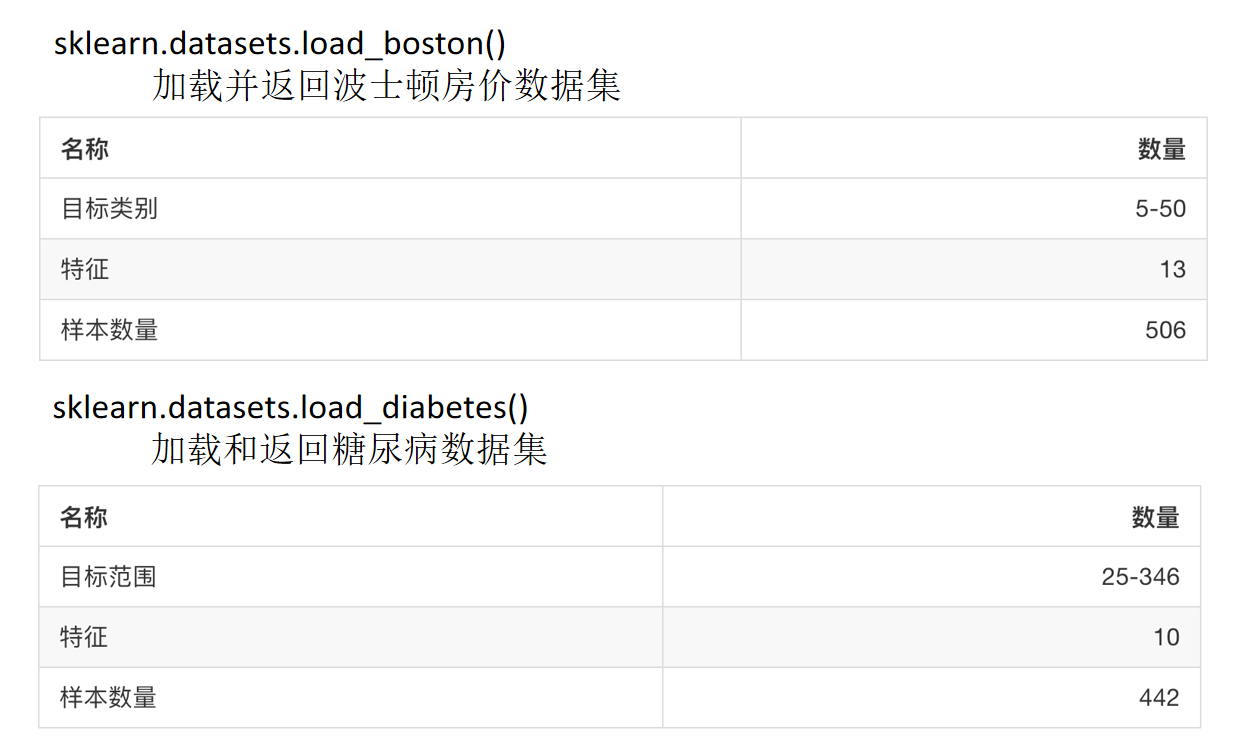
sklearn regression dataset

Converter and estimator

converter

In the previous feature engineering steps, the first step instantiates a transformer class, and the second step calls fit_ Transform (for the establishment of classification word frequency matrix for documents, it cannot be called at the same time)

fit_transform(): direct conversion of input data, equivalent to fit()+transform()

fit(): input data, take this data as the standard, but do not perform data conversion

transform(): perform data conversion according to the standard

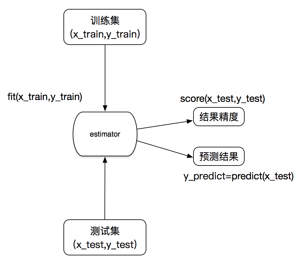
estimator

In sklearn, estimator plays an important role. Both classifier and regressor belong to estimator, which is a kind of API that implements the algorithm

1. Estimator for classification:

sklearn.neighbors k-nearest neighbor algorithm

sklearn.naive_bayes Bayes

sklearn.linear_model.LogisticRegression

1. Estimator for regression:

sklearn.linear_model.LinearRegression linear regression

sklearn.linear_model.Ridge ridge ridge regression

Workflow of estimator