Neural network is the basis of deep learning. The previous section mentioned that LR can connect to neural network. This section reviews and summarizes neural network and BP algorithm.
1. From LR to neural network
It was mentioned at the end of the logistic regression article that when the sample is linear and inseparable, the sample data needs to be transformed. After the transformation, the classification is carried out, and the transformation step becomes the process of feature extraction. The structure is shown in the figure:
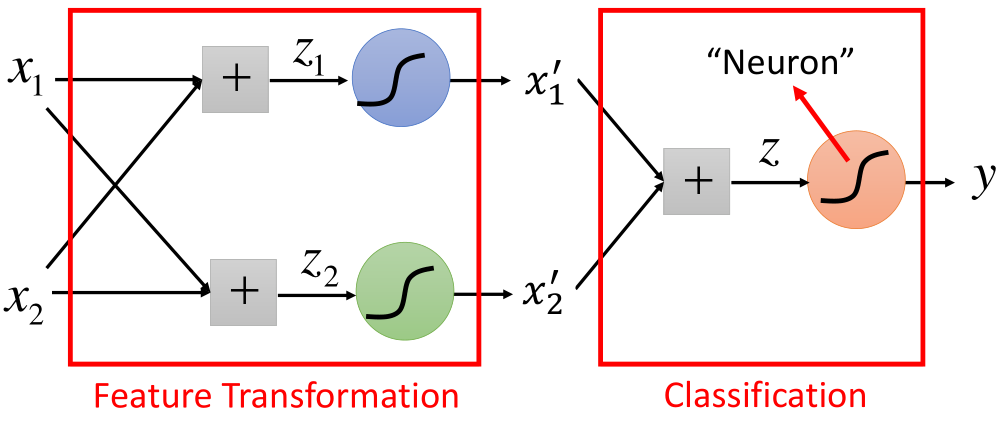
As shown in the above figure, each time the structure in the figure is converted, it is called a neuron. It can also have the following structures:

Similarly, a red framed part is called neuron. Different connection modes of neurons will produce different models, and the parameters of the model are contained in the neuron.
It is worth mentioning that in the previous LR, when the data are linearly separable, we need to find the equation of feature transformation to make the samples linearly separable, and then use LR for classification;
However, in the neural network, we do not need to find the transformed equation. The parameters are included in the network and trained together. At this time, we need to design the structure of the network to find out the appropriate model (parameters) and get good results.
2. Fully connected neural network
Network / model structure
According to the three-step theory of machine learning, first we need to determine the model, that is, what the model looks like. Here is a fully connected neural network.
The connection mode between neurons of neural network determines various models and structures of neural network. The following is the most common neural network structure - fully connected neural network:
As the name suggests, fully connected neural network means that each neuron is connected to each other. First, let's take a look at the propagation process of a structure through an example:
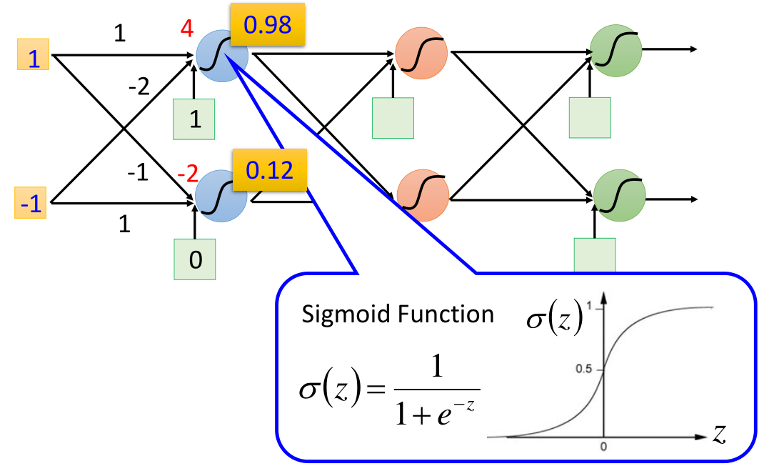
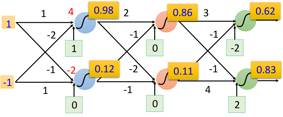
On the left is the input (1, - 1), each arrow points to the weight parameter w, and the green box is the deviation b. first, add linearly, and then pass through the sigmoid equation to obtain the output. After that, take the output as the input of the next propagation and move on:
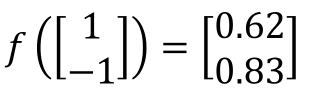
Then, the above process is expressed in vector form as:
Replace the neuron "neuron" in the box in Section 1 with "○", then the structure of the fully connected neural network is as follows:
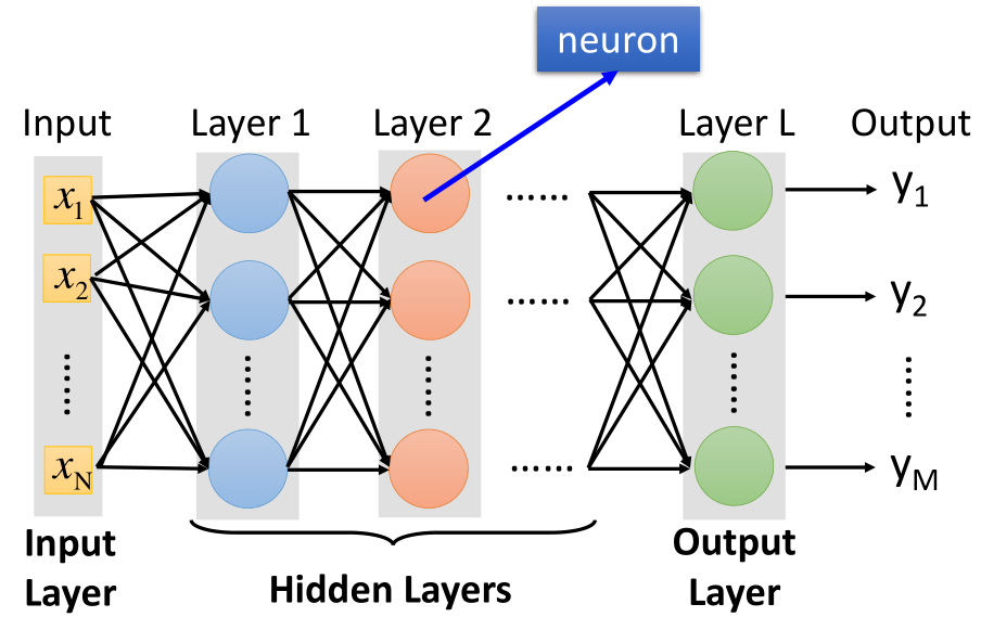
The above is a relatively complete fully connected neural network structure. The leftmost is the input, which is called the input layer, the rightmost is the output, which is called the output layer, and the structure between the input-output and output layers is called the hidden layer;
It is worth noting that in the neural network, the structure close to the input layer on the left is called "back", and the structure close to the output layer on the right is called "front". Therefore, the communication mode of the above example is also called forward communication.
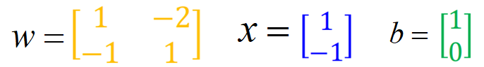
Then, the forward propagation process of the above example is expressed in the form of vector. Here, we only look at the process of the first layer:

The four weights in the first layer are expressed in the form of vectors:
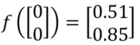
Then go through the sigmoid function:
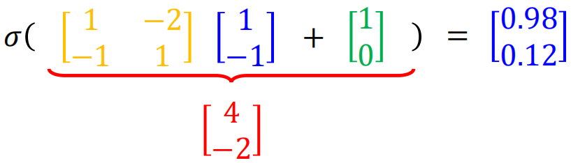
It can be seen that each neuron is actually an LR unit. In general, the vector form of forward propagation of neural network is:
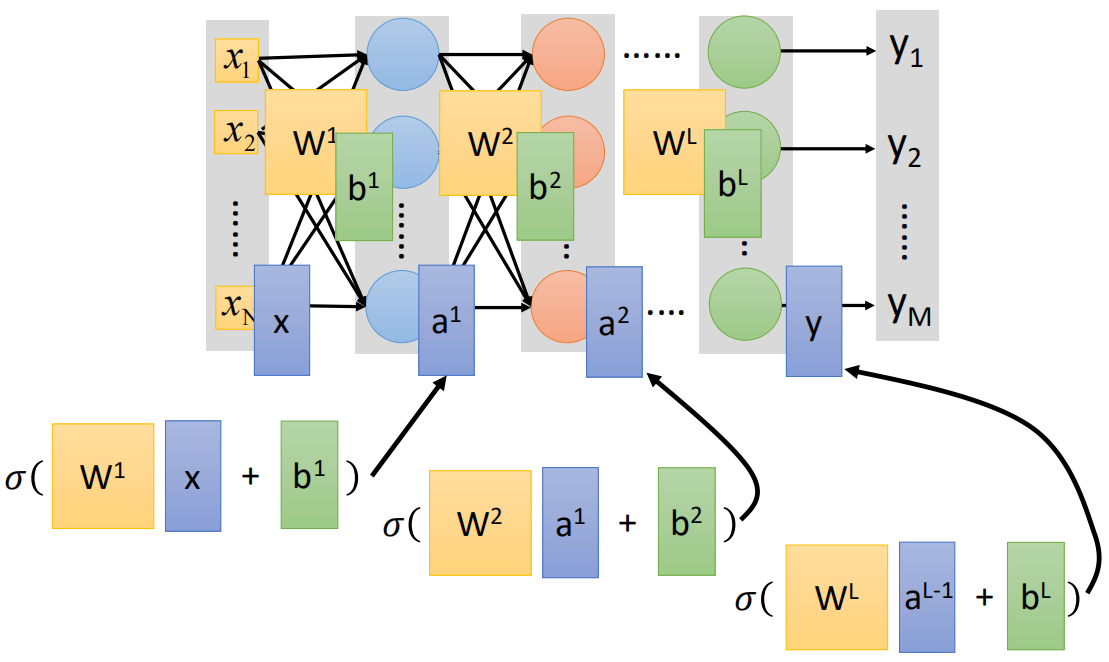
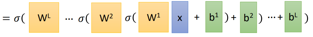
The output of each layer is the input of the next layer until the last output layer. The above is the forward propagation process of neural network.
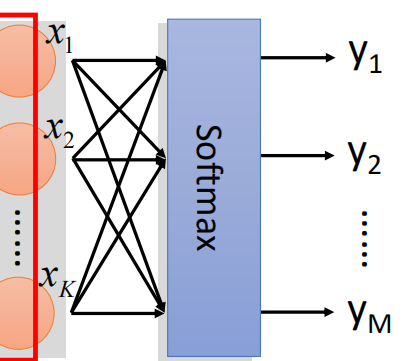
In the multi classification problem, the output layer of the last layer is usually the Softmax function for multi classification.
3. Model training and BP algorithm
The structure of the network needs to be given initially, that is, the number of layers of the network and the number of neurons contained in each network. If the structure of the network model is determined, the number of parameters is determined. Then the next step is to find the best set of parameters, that is, the training of the model.
According to the way we calculate the loss in LR, in the neural network, we also expect that the closer the real value is to the predicted value, the better. Therefore, the cross entropy is also used as the loss function here. The difference is that the derivation of cross entropy in LR comes from the derivation of maximum likelihood estimation, and the cross entropy formula is directly used here, The closer the real distribution of the expected sample is to the predicted distribution, the better, that is:
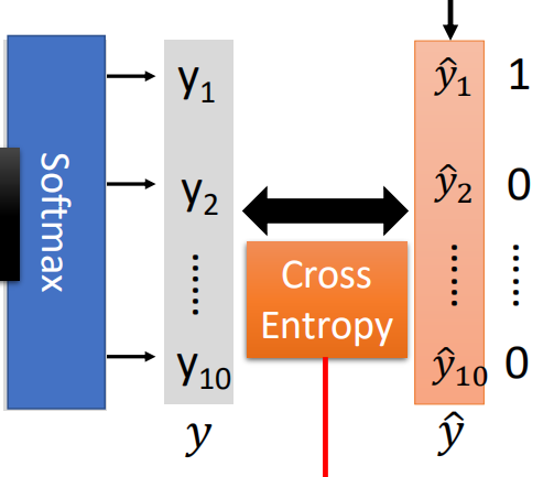
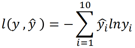
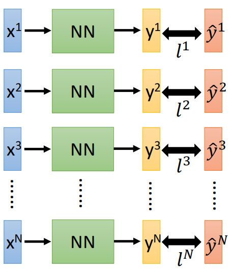
Here, assuming that the category of multi classification is 10 categories, it is necessary to calculate the cross entropy between each dimension, and then add it to obtain the cross entropy of a sample. For multiple samples, adding all samples again is the cross entropy loss function:
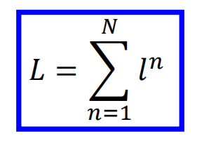
Then, the gradient descent is used to solve the problem, and the gradient is:
This gradient descent training method of forward propagation is consistent with the previous one. However, when the network is too complex, the number of parameters is too large, so the target loss function may be too complex and the direct derivation is difficult. Therefore, in order to calculate the gradient more effectively, BP back propagation algorithm is usually used.
Principle of BP algorithm
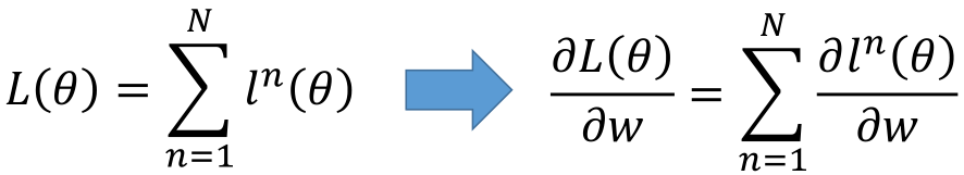
The loss function of neural network is L( θ), Then the derivative of the loss function to the parameter is:
First, take out a neuron:
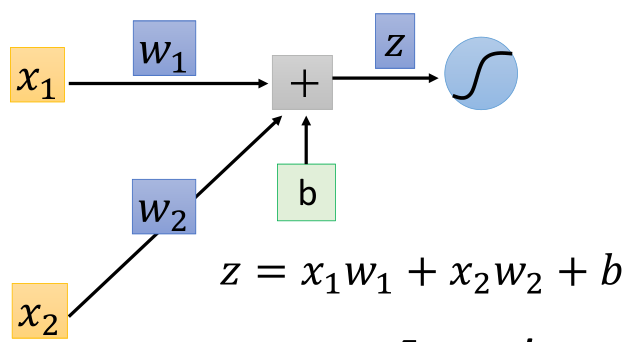
According to the chain derivation rule:

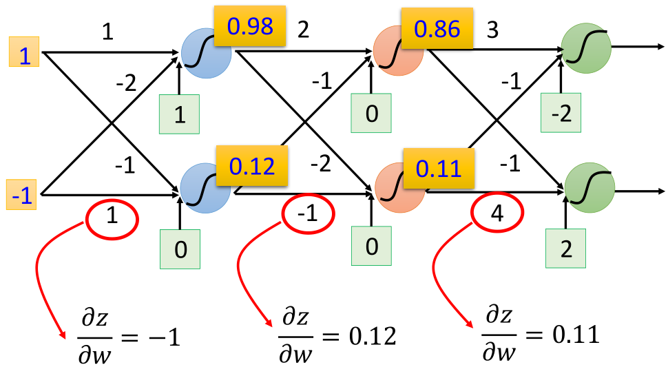
It can be seen here that the first part of the derivative, that is, the derivative of z to w, is the input x corresponding to w, such as the following example:
Next, look at the second half of the derivative obtained by chain derivation. Assuming that the output of this neuron is a, further use the chain derivation rule:
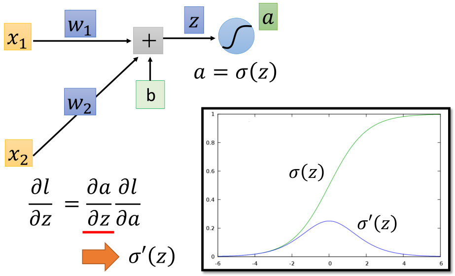
The first half of the derivative is the derivative of sigmoid function σ' (z) , and then the second half. a is the output of this layer and also the input of the network of the next layer. It is related to l, so continue to the next layer:
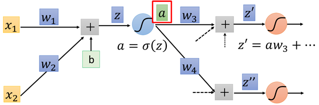
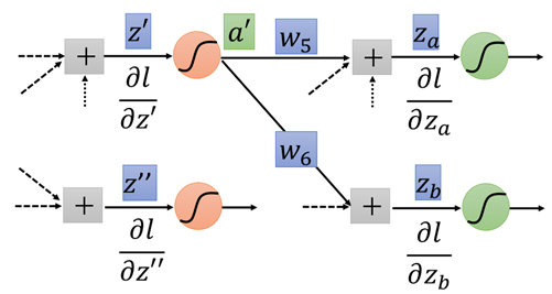
As the input of the following network, a affects each output of the next layer network. Assuming that there are two neurons in the next layer, then a is linearly weighted to obtain z 'and z' 'respectively, then according to the chain derivation rule:
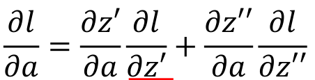
Two parts. The first half of each part is the weight w of the connection corresponding to input a, that is:
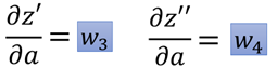 .
.
Then there are:
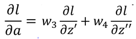
Then go back to the derivative of l over z in step 1:

If you reach the output layer at this step, you can know the derivatives of l to z 'and z' 'respectively, because:
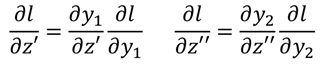
Then we can find the derivative of l over w.
If this step does not reach the output layer, continue to the next layer:
Continue to repeat the above steps until the output layer is reached.
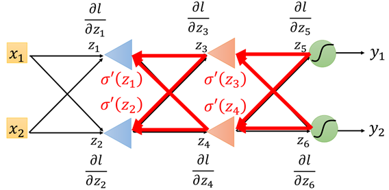
From the above process, we need to recursively calculate the derivative of l to z step by step until it propagates to the output layer, then calculate the derivative of output layer y to the previous layer, and then transfer it step by step backward (input layer). Finally, we get the derivative of l to w, that is, the gradient, and we can use the gradient descent for iteration.
Therefore, the above process is a back propagation process, as shown in the figure:
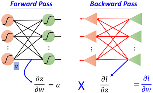
According to the above process, the first part of each term in the chain derivation result obtained by forward propagation is easier to be derived directly, and the second part of each term obtained by back propagation needs to be obtained recursively, as shown in the figure:
4. Using Keras to realize deep learning
The following is an example to realize neural network (deep learning) and illustrate the role of each step.
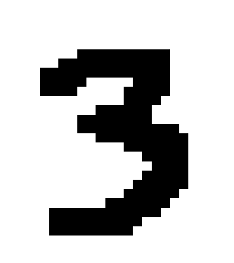
Firstly, the data set comes from MNIST handwritten numeral recognition data set. The data is handwritten picture data of 0 ~ 9. First, import the required library, read the data set from sklearn and process the data:
from sklearn.datasets import fetch_openml
from sklearn.preprocessing import OneHotEncoder
from sklearn.model_selection import train_test_split
import numpy as np
from keras import Sequential
from keras.layers import Dense
from keras.layers import Activation
import matplotlib.pyplot as plt
import matplotlib as mpl


data_x, data_y = fetch_openml('mnist_784', version=1, return_X_y=True)
# Set greater than 0 to 1, as long as the picture data of 0 and 1
data_x[data_x > 0] = 1

data_x = np.mat(data_x)

one_hot = OneHotEncoder()
data_y = one_hot.fit_transform(np.array(data_y).reshape(data_y.shape[0], 1)).toarray()

train_x, test_x, train_y, test_y = train_test_split(data_x, data_y)
Let's take a look at what data looks like:
data_x[:10]
####
matrix([[0., 0., 0., ..., 0., 0., 0.],
        [0., 0., 0., ..., 0., 0., 0.],
        [0., 0., 0., ..., 0., 0., 0.],
        ...,
        [0., 0., 0., ..., 0., 0., 0.],
        [0., 0., 0., ..., 0., 0., 0.],
        [0., 0., 0., ..., 0., 0., 0.]])

data_y[:10]
####
array([[0., 0., 0., 0., 0., 1., 0., 0., 0., 0.],
       [1., 0., 0., 0., 0., 0., 0., 0., 0., 0.],
       [0., 0., 0., 0., 1., 0., 0., 0., 0., 0.],
       [0., 1., 0., 0., 0., 0., 0., 0., 0., 0.],
       [0., 0., 0., 0., 0., 0., 0., 0., 0., 1.],
       [0., 0., 1., 0., 0., 0., 0., 0., 0., 0.],
       [0., 1., 0., 0., 0., 0., 0., 0., 0., 0.],
       [0., 0., 0., 1., 0., 0., 0., 0., 0., 0.],
       [0., 1., 0., 0., 0., 0., 0., 0., 0., 0.],
       [0., 0., 0., 0., 1., 0., 0., 0., 0., 0.]])
X is a 28 * 28 784 dimensional sparse matrix, and Y is a 10 dimensional data after independent heat coding. Let's draw any one:
def plot_digit(data):
    image = data.reshape(28, 28)
    plt.imshow(image, cmap=mpl.cm.binary, interpolation='nearest')
    plt.axis("off")


one_digit = data_x[10000]
plot_digit(one_digit)
After the data is ready, it comes to the modeling stage, which is modeled by using the keras neural network framework:
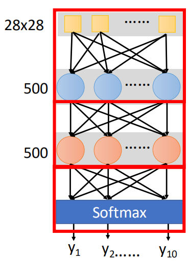
The first is the network structure. We need to determine a network structure ourselves, including the number of network layers and the number of neurons in each layer. Here, the input is 28 * 28 dimensions, so the input layer is 784 dimensions, the output is 10 dimensions and the output layer structure is 10 dimensions. The middle layer is tentatively set as 500, and the network structure is shown in the figure:
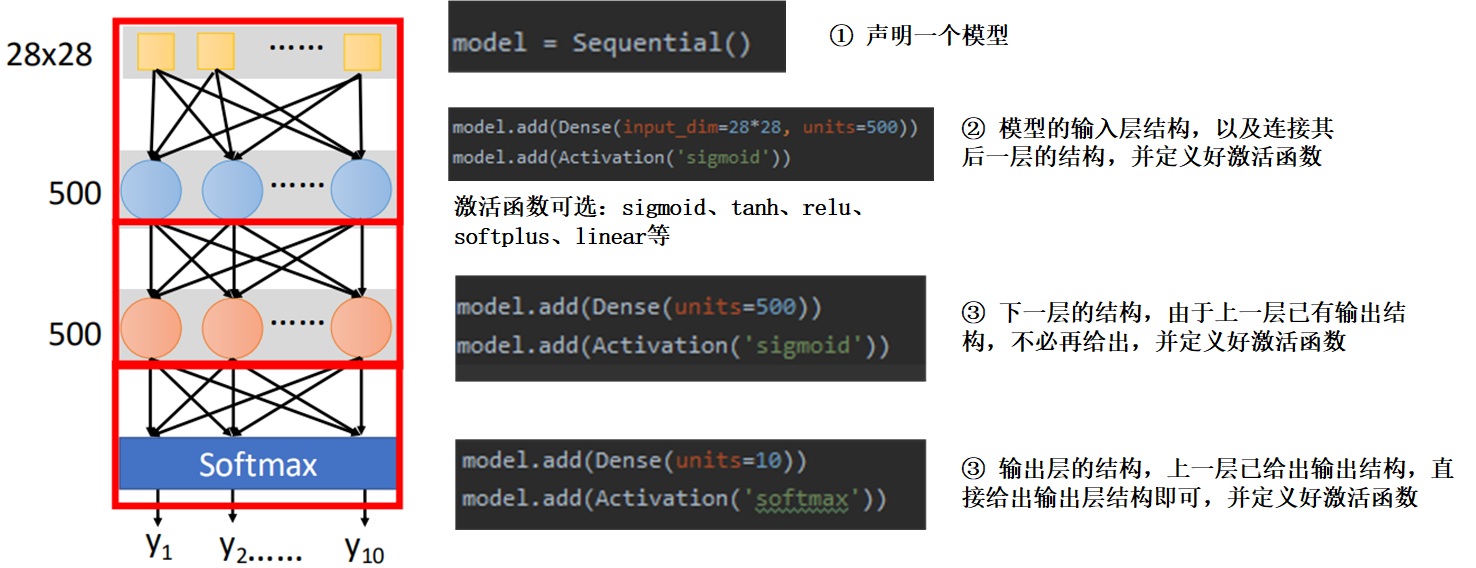
Then, we use keras to model the above network:
In this way, the model is built. The next step is to compile the model. This is different from the previous one. You can fit it by directly defining the model and parameters:
model.compile(optimizer='adam', loss='categorical_crossentropy', metrics=['accuracy'])
The optional optimizer is the parameter optimization method described in the previous gradient descent section. See the following for details: https://www.cnblogs.com/501731wyb/p/15322391.html
There are also many loss options. You can see the official documents: https://keras.io/zh/losses/.
Next, we used the data for training:
model.fit(train_x, train_y, batch_size=300, epochs=20)
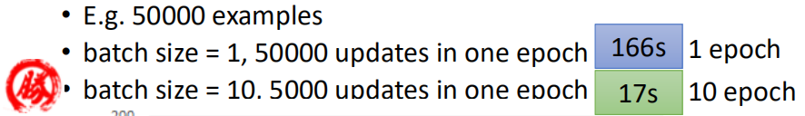
Here is batch_size is to use a batch of data for training, select one batch and continue to the next batch until all data are completed once and become an epoch.
Then view the training results and performance on the test set:
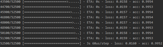
score = model.evaluate(test_x, test_y)
print('total loss on testing data', score[0])
print('accuracy on testing data', score[1])


32/17500 [..............................] - ETA: 17s
 1120/17500 [>.............................] - ETA: 1s
 2272/17500 [==>...........................] - ETA: 0s
 3648/17500 [=====>........................] - ETA: 0s
 5216/17500 [=======>......................] - ETA: 0s
 6720/17500 [==========>...................] - ETA: 0s
 8224/17500 [=============>................] - ETA: 0s
 9888/17500 [===============>..............] - ETA: 0s
11648/17500 [==================>...........] - ETA: 0s
13376/17500 [=====================>........] - ETA: 0s
15072/17500 [========================>.....] - ETA: 0s
16864/17500 [===========================>..] - ETA: 0s
17500/17500 [==============================] - 1s 35us/step
total loss on testing data 0.116816398623446
accuracy on testing data 0.9730285714285715
It can be seen that the accuracy is about 99.53 in the training set and 97.3% in the test set. There are 17500 pictures in the test data, of which 472 are misclassified. We find these 472:
error_idx = []
for i in range(len(test_x)):
    predict_array = model.predict(test_x[i])
    true_array = test_y[i]
    predict_result = np.argmax(predict_array)
    true_idx = np.argwhere(true_array == 1)[0][0]
    if true_idx != predict_result:
        error_idx.append(i)
Then look at the wrong data. First write a batch drawing function:
def plot_digits(instances, image_per_row=10, **options):
    size = 28
    image_per_row = min(len(instances), image_per_row)
    images = [instance.reshape(28, 28) for instance in instances]

    n_rows = (len(instances) - 1)//image_per_row + 1
    row_images = []
    n_empty = n_rows * image_per_row - len(instances)
    images.append(np.zeros((size, size * n_empty)))
    for row in range(n_rows):
        rimages = images[row*image_per_row:(row+1)*image_per_row]
        row_images.append(np.concatenate(rimages, axis=1))

    image = np.concatenate(row_images, axis=0)
    plt.imshow(image, cmap=mpl.cm.binary, **options)
    plt.axis("off")
    plt.figure(figsize=(9, 9))
Then draw some data and see why it is wrong:
example_images = []
for idx in error_idx[:30]:
    example_images.append(test_x[idx])

plot_digits(example_images, image_per_row=10)
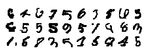
It can be seen from these pictures that most of the misdivided data are still difficult to distinguish. For example, the first one in the second row is difficult to distinguish with the naked eye.
This may be because the feature extraction is not enough, resulting in wrong classification. The model needs to be further adjusted. The next section mainly discusses some optimization strategies in deep learning.
Neural network has been preliminarily introduced here. It mainly introduces the fully connected neural network and BP algorithm, which is implemented by using the keras framework, and completes the "Hello World" of deep learning.
The content mainly comes from Mr. Li Hongyi's course. Since I've been watching it for a long time, I'll review it here. There are many things and it's finally over. The next section mainly summarizes the common loss functions and characteristics, as well as some model optimization and adjustment strategies in in-depth learning.