Scikit learn and Feature Engineering

"Data determines the upper limit of machine learning, and the algorithm only approximates this upper limit as much as possible". This sentence well expounds the importance of data in machine learning. Most of the data taken directly are not obvious, unprocessed, or there are a lot of useless data, so some feature processing and feature scaling are needed to meet the requirements of training data.

Scikit-learn

• Machine learning tools for Python language
• Applicable to everyone and can be reused in different contexts
• Built based on NumPy, SciPy and matplotlib
• Open source, commercially available - BSD license

Feature Engineering of data

• The useful information extracted from the data for the prediction results is processed through professional skills, so that the features can play a better role in the machine learning algorithm.
• High quality features often describe the inherent structure of data. The initial original feature data set may be too large or information redundant. Therefore, in the application of machine learning, an initial step is to select a subset of features or build a new set of features to reduce functions to promote the learning of the algorithm and improve the generalization ability and interpretability.

Significance of Feature Engineering

• Better features mean stronger robustness
• Better features mean that only simple models are needed
• Better features mean better results

Feature processing of Feature Engineering

The most important part of feature engineering is feature processing, which contains many specific professional skills

• Feature preprocessing
  • Single feature
    • normalization
    • Standardization
    • Missing value
  • Multiple features
    • Dimensionality reduction
    • PCA

Feature extraction and feature selection in Feature Engineering

If we say that feature processing is actually calculating the existing data to achieve our target data standard. Feature extraction is to convert any data format (such as text and image) into digital features of machine learning. Feature selection is to select better features from the existing features.

Source and type of data

Most of the data comes from the existing database. If not, it can also be collected and provided by many crawler engineers. It can also come from the usual records. Anyway, the data is everywhere and most of them are available

Type of data

According to the data classification of machine learning, we can divide the data into:

• Nominal type: the results of nominal type target variables only take values in limited target sets, such as true and false (nominal type target variables are mainly used for classification)
• Numerical type: numerical type target variables can be taken from an infinite set of values, such as 0.100, 42.001, etc. (numerical type target variables are mainly used for regression analysis)

According to the distribution characteristics of the data itself

• Discrete type
• Continuous type

So what are discrete and continuous data? Firstly, continuous data is regular, while discrete data is irregular

• Discrete variables refer to discrete variables whose values can only be calculated in natural or integer units, such as class number, number of goals, whether it is a category, etc
• Continuous data refers to any value within a specified interval, such as box office data and petal size distribution data
• The discrete type is inseparable within the interval, and the continuous type is separable within the interval

Feature extraction of data

In the real world, most features are not continuous variables, such as classification, text, image, etc. in order to express the features of discontinuous variables, these features need to be mathematically expressed, so feature extraction. Sklearn.feature is used_ Extraction provides many methods of feature extraction

Classification feature variable extraction

Dictionary feature extraction

We use city and environment as dictionary data to extract features.

DictVectorizer syntax

DictVectorizer.fit_transform(X)       
	X:Dictionary or iterator containing dictionary
	Return value: Return sparse matrix
DictVectorizer.inverse_transform(X)
	X:array Array or sparse matrix
	Return value:Data format before conversion
DictVectorizer.get_feature_names()
	Return category name
DictVectorizer.transform(X)
	Convert according to the original standard

technological process:

1. Instantiate class DictVectorizer
2. Call fit_ The transform method inputs data and transforms it. Note the return format

method

fit_transform(X,y)

Apply and convert the mapping list X, y to the target type

inverse_transform(X[, dict_type])

Converts a Numpy array or a scipy.spark matrix to a mapping list

from sklearn.feature_extraction import DictVectorizer
onehot = DictVectorizer() # If the result does not use toarray, please turn on spark = false
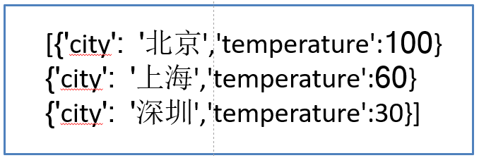
instances = [{'city': 'Beijing','temperature':100},{'city': 'Shanghai','temperature':60}, {'city': 'Shenzhen','temperature':30}]
X = onehot.fit_transform(instances).toarray()
print(onehot.inverse_transform(X))

Text feature extraction (English only)

Text feature extraction is used in many aspects, such as document classification, spam classification and news classification. Then text classification is expressed by the existence of words and the probability (importance) of words.

(1) Appearance of words in documents

A value of 1 indicates that the word in the thesaurus appears, and a value of 0 indicates that it does not appear

sklearn.feature_extraction.text.CountVectorizer()

Convert a collection of text documents into a counting matrix (SciPy. Spark matrices)

method

fit_transform(raw_documents,y)

Learn the vocabulary dictionary and return to the vocabulary document matrix

from sklearn.feature_extraction.text import CountVectorizer
content = ["life is short,i like python","life is too long,i dislike python"]
vectorizer = CountVectorizer()
print(vectorizer.fit_transform(content).toarray())

The toarray() method needs to be converted to the array form of numpy

Warm tip: the words in each document are only a small part of all the words in the whole corpus, resulting in the sparsity of feature vectors (many values are 0). In order to solve the problem of storage and operation speed, Python's scipy.spark matrix structure is used

(2) Importance of TF-IDF expression

TfidfVectorizer converts the words in the document into probability representation according to the specified formula. (naive Bayes introduces detailed usage)

class sklearn.feature_extraction.text.TfidfVectorizer()

method

fit_transform(raw_documents,y)

Learn vocabulary and idf, and return to the term document matrix.

from sklearn.feature_extraction.text import TfidfVectorizer
content = ["life is short,i like python","life is too long,i dislike python"]
vectorizer = TfidfVectorizer(stop_words='english')
print(vectorizer.fit_transform(content).toarray())
print(vectorizer.vocabulary_)

Data feature preprocessing

Single feature

normalization

Firstly, when there are many features (dimensions), normalization can prevent a one-dimensional or several dimensions from having too much impact on the data. It is also to unify the data from different sources into a reference interval, which is meaningful for comparison. Secondly, the program can run faster. For example, a person's height and weight are two characteristics. If the weight is 50kg and the height is 175cm, the values are different because the two units are different. If we compare the body shape difference between two people, the influence of height will be greater, and the k-nearest neighbor algorithm will have this distance formula.

Min max method

Here we use the data of blind date in MatchData.txt, which is the data of men in this sample. There are three characteristics: the percentage of time spent playing games, the frequent flyer mileage obtained every year, and the litres of ice cream consumed every week. Then there is a category, three categories evaluated by women, dislike, general charm and great charm. First, import data for matrix conversion

import numpy as np

def data_matrix(file_name):
  """
  Convert text to matrix
  :param file_name: file name
  :return: Data matrix
  """
  fr = open(file_name)
  array_lines = fr.readlines()
  number_lines = len(array_lines)
  return_mat = zeros((number_lines, 3))
  # classLabelVector = []
  index = 0
  for line in array_lines:
    line = line.strip()
    list_line = line.split('\t')
    return_mat[index,:] = list_line[0:3]
    # if(listFromLine[-1].isdigit()):
    #     classLabelVector.append(int(listFromLine[-1]))
    # else:
    #     classLabelVector.append(love_dictionary.get(listFromLine[-1]))
    # index += 1
  return return_mat

Output results

[[  4.09200000e+04   8.32697600e+00   9.53952000e-01]
 [  1.44880000e+04   7.15346900e+00   1.67390400e+00]
 [  2.60520000e+04   1.44187100e+00   8.05124000e-01]
 ...,
 [  2.65750000e+04   1.06501020e+01   8.66627000e-01]
 [  4.81110000e+04   9.13452800e+00   7.28045000e-01]
 [  4.37570000e+04   7.88260100e+00   1.33244600e+00]]

When we look at the data set, we find that some values are as large as tens of thousands and some are only single digits. Similarly, when calculating the distance between two samples, one of them will have a great impact. In other words, flight mileage has a great impact on settlement results or blind date results, but statisticians think these three characteristics are equally important, so they need to process the data in this way.

In this way, the arbitrary range of each feature will become the value in the interval of [0,1], or it can be processed to [- 1,1] according to the requirements. We define a function to carry out such conversion.

def feature_normal(data_set):
    """
    feature normalization 
    :param data_set:
    :return:
    """
    # Minimum value per column
    min_vals = data_set.min(0)
    # Maximum value per column
    max_vals = data_set.max(0)
    ranges = max_vals - min_vals
    norm_data = np.zeros(np.shape(data_set))
    # Number of trips
    m = data_set.shape[0]
    # Matrix subtraction
    norm_data = data_set - np.tile(min_vals, (m,1))
    # Matrix Division
    norm_data = norm_data/np.tile(ranges, (m, 1)))
    return norm_data

The output result is

[[ 0.44832535  0.39805139  0.56233353]
 [ 0.15873259  0.34195467  0.98724416]
 [ 0.28542943  0.06892523  0.47449629]
 ...,
 [ 0.29115949  0.50910294  0.51079493]
 [ 0.52711097  0.43665451  0.4290048 ]
 [ 0.47940793  0.3768091   0.78571804]]

The class MinMaxScaler in scikit-learn.preprocessing scales the data matrix between [0,1]

>>> X_train = np.array([[ 1., -1.,  2.],
...                     [ 2.,  0.,  0.],
...                     [ 0.,  1., -1.]])
...
>>> min_max_scaler = preprocessing.MinMaxScaler()
>>> X_train_minmax = min_max_scaler.fit_transform(X_train)
>>> X_train_minmax
array([[ 0.5       ,  0.        ,  1.        ],
       [ 1.        ,  0.5       ,  0.33333333],
       [ 0.        ,  1.        ,  0.        ]])

Note that the maximum and minimum values change in specific scenarios. In addition, the maximum and minimum values are very vulnerable to outliers, so this method has poor robustness and is only suitable for traditional accurate small data scenarios

Standardization

The commonly used method is z-score standardization. After processing, the mean value of the data is 0 and the standard deviation is 1

They can be estimated by existing samples, which are stable when there are enough samples, and are suitable for noisy data scenes
The StandardScalar class is provided in sklearn to standardize columns:

In [2]: import numpy as np
In [3]: X_train = np.array([[ 1., -1.,  2.],[ 2.,  0.,  0.],[ 0.,  1., -1.]])
In [4]: from sklearn.preprocessing import StandardScaler
In [5]: std = StandardScaler()
In [6]: X_train_std = std.fit_transform(X_train)
In [7]: X_train_std
Out[7]:
array([[ 0.        , -1.22474487,  1.33630621],
       [ 1.22474487,  0.        , -0.26726124],
       [-1.22474487,  1.22474487, -1.06904497]])

Missing value

For various reasons, many real-world datasets contain missing values, usually encoded as blanks, NaN, or other placeholders. However, such data sets are not compatible with scikit's classifier. They assume that all values in the array are numbers and have and hold meanings. The basic strategy for using incomplete datasets is to discard entire rows and / or columns that contain missing values. However, this comes at the cost of losing data that may be valuable, even if incomplete. A better strategy is to estimate missing values, that is, infer them from known parts of the data.
(1) Fill in the missing values. Use the Imputer class in sklearn.preprocessing to fill in the data

class Imputer(sklearn.base.BaseEstimator, sklearn.base.TransformerMixin)
    """
    Used to complete the supplement of missing values

    :param param missing_values: integer or "NaN", optional (default="NaN")
        Placeholder for missing value for encoding np.nan Missing value for, use string value“ NaN"

    :param strategy: string, optional (default="mean")
        Interpolation strategy
        If it is average, replace the missing value with the average along the axis
        If median, replace the missing value with the median along the axis
        If“ most_frequent"，Then replace the missing value with the most frequent value along the axis

    :param axis: integer, optional (default=0)
        Interpolated axis
        If axis = 0，Then arrange along the column
        If axis = 1，Then arrange along the line
    """

Multiple features

Dimensionality reduction

PCA (Principal component analysis) is characterized by saving those features that have the greatest impact on each other's difference in the data set. PCA is extremely vulnerable to the range of features in the data, so it is necessary to standardize the features before using PCA, so as to ensure the equal importance of features in each dimension

sklearn.decomposition.PCA

class PCA(sklearn.decomposition.base)
   """
   Principal component analysis

   :param n_components: int, float, None or string
       This parameter can help us specify the desired value PCA The number of feature dimensions after dimension reduction. The most common method is to directly specify the number of dimensions to be reduced. At this time n_components Is an integer greater than 1.
       We can also use the default value, that is, no input n_components，here n_components=min(Number of samples)

   :param whiten: bool, optional (default False)
      Judge whether to whiten. The so-called whitening is to normalize each feature of the data after dimensionality reduction PCA Dimension reduction itself generally does not require whitening,If you PCA There are subsequent data processing actions after dimension reduction. Whitening can be considered. The default value is False，That is, no whitening

   :param svd_solver:
      Choose an appropriate SVD Algorithm to reduce dimension,In general, using default values is sufficient.
    """

example

>>> import numpy as np
>>> from sklearn.decomposition import PCA
>>> X = np.array([[-1, -1], [-2, -1], [-3, -2], [1, 1], [2, 1], [3, 2]])
>>> pca = PCA(n_components=2)
>>> pca.fit(X)
PCA(copy=True, iterated_power='auto', n_components=2, random_state=None,
  svd_solver='auto', tol=0.0, whiten=False)
>>> print(pca.explained_variance_ratio_)
[ 0.99244...  0.00755...]

Feature selection of data

Dimensionality reduction is essentially mapping from one dimension space to another. The number of features does not decrease. Of course, the feature value will change accordingly in the process of mapping. For example, the current feature is 1000 dimensions, and we want to reduce it to 500 dimensions. The process of dimensionality reduction is to find a mapping relationship from 1000 dimensions to 500 dimensions. 1000 features in the original data , each corresponds to a value in the 500 dimensional space after dimension reduction. Assuming that the value of one feature in the original feature is 9, the corresponding value after dimension reduction may be 3. For feature selection, there are many methods:

• Filter: VarianceThreshold
• Embedded: regularization, decision tree
• Wrapper (wrapped)

sklearn.feature_selection

Remove the feature with small value change (delete the low variance feature)

VarianceThreshold is a basic method in feature selection. It removes all features whose variance does not meet the threshold. By default, it removes all features with variance of 0, that is, those with exactly the same value in all samples.

Suppose we want to remove features where more than 80% of the data is 1 or 0

from sklearn.feature_selection import VarianceThreshold
X = [[0, 0, 1], [0, 1, 0], [1, 0, 0], [0, 1, 1], [0, 1, 0], [0, 1, 1]]
sel = VarianceThreshold(threshold=(.8 * (1 - .8)))
sel.fit_transform(X)
array([[0, 1],
       [1, 0],
       [0, 0],
       [1, 1],
       [1, 0],
       [1, 1]])