[GNN benchmark] Figure benchmark data set of machine learning

Figure ImageNet of neural network? Open source millions of OGB benchmark data sets such as Stanford University

In the small data full of "MNIST", does graph neural network also need a big benchmark such as "ImageNet"? Recently, Professor Jure Leskovec of Stanford University announced the open source of Open Graph Benchmark in a speech at the neurps 2019 conference, which is an important step towards a unified benchmark for graph neural network modeling.

Reprint:

The heart of official account machine Figure ImageNet of neural network? Stanford University and other open source millions of OGB benchmark data sets - know

official account

Graph neural network is a rapidly developing branch of machine learning. By transforming unstructured data into structured graphs of nodes and edges, and then using graph neural network for learning, we can often achieve better results.

However, up to now, there is no recognized benchmark data set for graph neural network. The methods used in many papers are often aimed at small data sets that lack node and edge features. Therefore, the model performance obtained on these data sets is difficult to be said to be the best and not necessarily reliable, which hinders further development.

In the graph representation learning speech at the neurps 2019 conference, Jure Leskovec announced the general performance evaluation benchmark data set OGB (Open Graph Benchmark) of open source graph neural network. Through this data set, we can better evaluate the indicators of model performance and so on.

Project address: http://ogb.stanford.edu
The figure shows the collection of learning speeches: https://slideslive.com/38921872/graph-representation-learning-3

The guest speaker of this speech is Jure Leskovec, an associate professor of computer science at Stanford University. His main research interests are mining and modeling of social information networks, especially for large-scale data, network and media data.

It is worth noting that OGB dataset also supports PYG and DGL, two commonly used graph neural network frameworks. One of the sponsors of DGL project and President of AWS Shanghai AI research institute, Professor Zhang Zheng of New York University in Shanghai (during academic leave) said: "At this stage, I think the greatest role of OGB is to promote the academic community to go out of the toy data set. A unified, more complex and more diverse data set enables researchers to gather strength again. Although there will be disadvantages caused by model over fitting the standard data set, it plays an important role in improving the effect of model and algorithm and the ability of DGL and other platforms."

Professor Zhang Zheng said that Open Graph Benchmark, a diverse and unified benchmark, is a very necessary step for graph neural network.

1.OGB

1.1 Overview

Open Graph Benchmark (hereinafter referred to as OGB) is an open source Python Library of Stanford University students. It contains the benchmark data set, data loader and evaluator of graph machine learning (hereinafter referred to as graph ML). Its purpose is to promote the research of scalable, robust and reproducible graph ML.

OGB contains many tasks of machine learning, and covers various fields from social and information networks to biological networks, molecular graphs and knowledge graphs. No data set has specific data splitting and evaluation indicators, so as to provide a unified evaluation protocol.

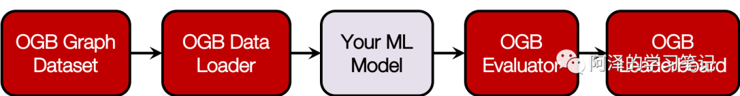
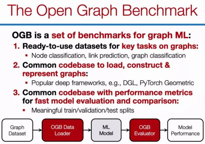
OGB provides an automatic pipeline of end-to-end graph ML, which simplifies and standardizes the process of graph data loading, experimental setting and model evaluation. As shown in the figure below:

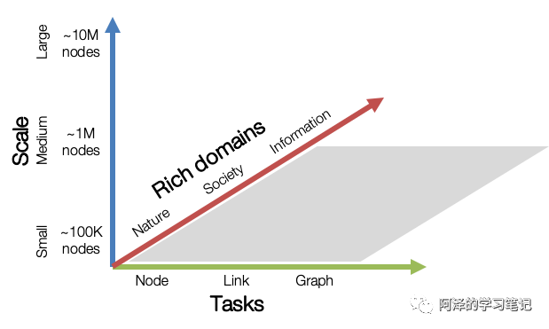
The following figure shows the three dimensions of OGB, including Tasks, Scale and Rich domains.

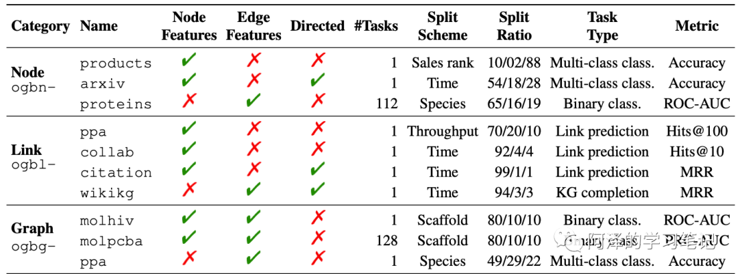
1.2 Dataset

Take a look at the data set that OGB now contains:

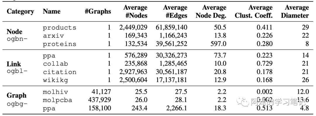
Statistical details of data sets:

1.3 Leaderboard

OGB also provides standardized assessors and leaderboards to track the latest results. Let's take a look at some leaderboards under different tasks.

Node classification: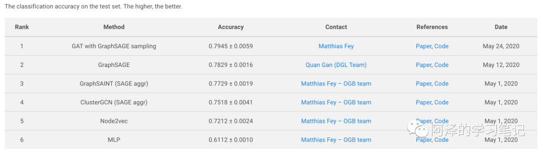

Link forecast: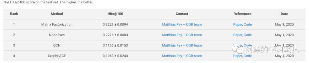

Figure classification:

2.OGB+DGL

The official examples are based on PyG. Here we implement an example based on DGL.

2.1 environmental preparation

Import package

import dgl
import ogb
import math
import time
import numpy as np
import torch
import torch.nn as nn
import torch.nn.functional as F
from ogb.nodeproppred import DglNodePropPredDataset, Evaluator

View version

print(dgl.__version__)
print(torch.__version__)
print(ogb.__version__)

0.4.3post2
1.5.0+cu101
1.1.1

cuda related information

print(torch.version.cuda)
print(torch.cuda.is_available())
print(torch.cuda.device_count())
print(torch.cuda.get_device_name(0))
print(torch.cuda.current_device())

10.1
True
1
Tesla P100-PCIE-16GB
0

2.2 data preparation

Set parameters

device_id=0  #Usage id of GPU #
n_layers=3  #Number of input layers + hidden layers + output layers
n_hiddens=256  #Number of hidden layer nodes
dropout=0.5
lr=0.01
epochs=300
runs=10  #Run 10 times and take the average
log_steps=50

Define training function, test function and log record

def train(model, g, feats, y_true, train_idx, optimizer):
    """ Training function
    """
    model.train()
    optimizer.zero_grad()
    out = model(g, feats)[train_idx]
    loss = F.nll_loss(out, y_true.squeeze(1)[train_idx])
    loss.backward()
    optimizer.step()

    return loss.item()


@torch.no_grad()
def test(model, g, feats, y_true, split_idx, evaluator):
    """ Test function
    """
    model.eval()

    out = model(g, feats)
    y_pred = out.argmax(dim=-1, keepdim=True)

    train_acc = evaluator.eval({
        'y_true': y_true[split_idx['train']],
        'y_pred': y_pred[split_idx['train']],
    })['acc']
    valid_acc = evaluator.eval({
        'y_true': y_true[split_idx['valid']],
        'y_pred': y_pred[split_idx['valid']],
    })['acc']
    test_acc = evaluator.eval({
        'y_true': y_true[split_idx['test']],
        'y_pred': y_pred[split_idx['test']],
    })['acc']

    return train_acc, valid_acc, test_acc

class Logger(object):
    """ For logging
    """
    def __init__(self, runs, info=None):
        self.info = info
        self.results = [[] for _ in range(runs)]

    def add_result(self, run, result):
        assert len(result) == 3
        assert run >= 0 and run < len(self.results)
        self.results[run].append(result)

    def print_statistics(self, run=None):
        if run is not None:
            result = 100 * torch.tensor(self.results[run])
            argmax = result[:, 1].argmax().item()
            print(f'Run {run + 1:02d}:')
            print(f'Highest Train: {result[:, 0].max():.2f}')
            print(f'Highest Valid: {result[:, 1].max():.2f}')
            print(f'  Final Train: {result[argmax, 0]:.2f}')
            print(f'   Final Test: {result[argmax, 2]:.2f}')
        else:
            result = 100 * torch.tensor(self.results)

            best_results = []
            for r in result:
                train1 = r[:, 0].max().item()
                valid = r[:, 1].max().item()
                train2 = r[r[:, 1].argmax(), 0].item()
                test = r[r[:, 1].argmax(), 2].item()
                best_results.append((train1, valid, train2, test))

            best_result = torch.tensor(best_results)

            print(f'All runs:')
            r = best_result[:, 0]
            print(f'Highest Train: {r.mean():.2f} ± {r.std():.2f}')
            r = best_result[:, 1]
            print(f'Highest Valid: {r.mean():.2f} ± {r.std():.2f}')
            r = best_result[:, 2]
            print(f'  Final Train: {r.mean():.2f} ± {r.std():.2f}')
            r = best_result[:, 3]
            print(f'   Final Test: {r.mean():.2f} ± {r.std():.2f}')

Load data

device = f'cuda:{device_id}' if torch.cuda.is_available() else 'cpu'
device = torch.device(device)

#Load data, name = ogbn - + dataset name
#You can print out {dataset} and have a look
dataset = DglNodePropPredDataset(name='ogbn-arxiv')
split_idx = dataset.get_idx_split()
g, labels = dataset[0]
feats = g.ndata['feat']
g = dgl.to_bidirected(g)
feats, labels = feats.to(device), labels.to(device)
train_idx = split_idx['train'].to(device)

2.3 GCN

To realize a basic GCN, a Batch Normalization is carried out for each layer. If it is removed, the accuracy will be reduced by about 2%.

from dgl.nn import GraphConv

class GCN(nn.Module):
    def __init__(self,
                 in_feats,
                 n_hiddens,
                 n_classes,
                 n_layers,
                 dropout):
        super(GCN, self).__init__()

        self.layers = nn.ModuleList()
        self.bns = nn.ModuleList()
        self.layers.append(GraphConv(in_feats, n_hiddens, 'both'))
        self.bns.append(nn.BatchNorm1d(n_hiddens))
        for _ in range(n_layers - 2):
            self.layers.append(GraphConv(n_hiddens, n_hiddens, 'both'))
            self.bns.append(nn.BatchNorm1d(n_hiddens))
        self.layers.append(GraphConv(n_hiddens, n_classes, 'both'))
        self.dropout = dropout

    def reset_parameters(self):
        for layer in self.layers:
            layer.reset_parameters()
        for bn in self.bns:
            bn.reset_parameters()

    def forward(self, g, x):
        for i, layer in enumerate(self.layers[:-1]):
            x = layer(g, x)
            x = self.bns[i](x)
            x = F.relu(x)
            x = F.dropout(x, p=self.dropout, training=self.training)
        x = self.layers[-1](g, x)
        return x.log_softmax(dim=-1)

model = GCN(in_feats=feats.size(-1),
            n_hiddens=n_hiddens,
            n_classes=dataset.num_classes,
            n_layers=n_layers,
            dropout=dropout).to(device)

evaluator = Evaluator(name='ogbn-arxiv')
logger = Logger(runs)

for run in range(runs):
    model.reset_parameters()
    optimizer = torch.optim.Adam(model.parameters(), lr=lr)
    for epoch in range(1, 1 + epochs):
        loss = train(model, g, feats, labels, train_idx, optimizer)
        result = test(model, g, feats, labels, split_idx, evaluator)
        logger.add_result(run, result)

        if epoch % log_steps == 0:
            train_acc, valid_acc, test_acc = result
            print(f'Run: {run + 1:02d}, '
                  f'Epoch: {epoch:02d}, '
                  f'Loss: {loss:.4f}, '
                  f'Train: {100 * train_acc:.2f}%, '
                  f'Valid: {100 * valid_acc:.2f}% '
                  f'Test: {100 * test_acc:.2f}%')

    logger.print_statistics(run)
logger.print_statistics()

Run: 01, Epoch: 50, Loss: 1.1489, Train: 68.71%, Valid: 68.93% Test: 68.32%
Run: 01, Epoch: 100, Loss: 1.0565, Train: 71.29%, Valid: 69.61% Test: 68.03%
Run: 01, Epoch: 150, Loss: 1.0010, Train: 72.28%, Valid: 70.57% Test: 70.00%
Run: 01, Epoch: 200, Loss: 0.9647, Train: 73.18%, Valid: 69.79% Test: 67.97%
Training time/epoch 0.2617543590068817
Run 01:
Highest Train: 73.54
Highest Valid: 71.16
  Final Train: 73.08
   Final Test: 70.43
Run: 02, Epoch: 50, Loss: 1.1462, Train: 68.83%, Valid: 68.69% Test: 68.50%
Run: 02, Epoch: 100, Loss: 1.0583, Train: 71.17%, Valid: 69.54% Test: 68.06%
Run: 02, Epoch: 150, Loss: 1.0013, Train: 71.98%, Valid: 69.71% Test: 68.06%
Run: 02, Epoch: 200, Loss: 0.9626, Train: 73.23%, Valid: 69.76% Test: 67.79%
Training time/epoch 0.26154680013656617
Run 02:
Highest Train: 73.34
Highest Valid: 70.87
  Final Train: 72.56
   Final Test: 70.42
Run: 03, Epoch: 50, Loss: 1.1508, Train: 68.93%, Valid: 68.49% Test: 67.14%
Run: 03, Epoch: 100, Loss: 1.0527, Train: 70.90%, Valid: 69.75% Test: 68.77%
Run: 03, Epoch: 150, Loss: 1.0042, Train: 72.54%, Valid: 70.71% Test: 69.36%
Run: 03, Epoch: 200, Loss: 0.9679, Train: 73.13%, Valid: 69.92% Test: 68.05%
Training time/epoch 0.26173179904619853
Run 03:
Highest Train: 73.44
Highest Valid: 71.04
  Final Train: 73.06
   Final Test: 70.53
Run: 04, Epoch: 50, Loss: 1.1507, Train: 69.02%, Valid: 68.81% Test: 68.09%
Run: 04, Epoch: 100, Loss: 1.0518, Train: 71.30%, Valid: 70.19% Test: 68.78%
Run: 04, Epoch: 150, Loss: 0.9951, Train: 72.05%, Valid: 68.20% Test: 65.38%
Run: 04, Epoch: 200, Loss: 0.9594, Train: 72.98%, Valid: 70.47% Test: 69.26%
Training time/epoch 0.2618525844812393
Run 04:
Highest Train: 73.34
Highest Valid: 70.88
  Final Train: 72.86
   Final Test: 70.60
Run: 05, Epoch: 50, Loss: 1.1500, Train: 68.82%, Valid: 69.00% Test: 68.47%
Run: 05, Epoch: 100, Loss: 1.0566, Train: 71.13%, Valid: 70.15% Test: 69.47%
Run: 05, Epoch: 150, Loss: 0.9999, Train: 72.48%, Valid: 70.88% Test: 70.27%
Run: 05, Epoch: 200, Loss: 0.9648, Train: 73.37%, Valid: 70.51% Test: 68.96%
Training time/epoch 0.261941517829895
Run 05:
Highest Train: 73.37
Highest Valid: 70.93
  Final Train: 72.77
   Final Test: 70.24
Run: 06, Epoch: 50, Loss: 1.1495, Train: 69.00%, Valid: 68.76% Test: 67.89%
Run: 06, Epoch: 100, Loss: 1.0541, Train: 71.24%, Valid: 69.74% Test: 68.21%
Run: 06, Epoch: 150, Loss: 0.9947, Train: 71.89%, Valid: 69.81% Test: 69.77%
Run: 06, Epoch: 200, Loss: 0.9579, Train: 73.45%, Valid: 70.50% Test: 69.60%
Training time/epoch 0.2620268513758977
Run 06:
Highest Train: 73.70
Highest Valid: 70.97
  Final Train: 73.70
   Final Test: 70.12
Run: 07, Epoch: 50, Loss: 1.1544, Train: 68.93%, Valid: 68.81% Test: 67.97%
Run: 07, Epoch: 100, Loss: 1.0562, Train: 71.17%, Valid: 69.79% Test: 68.45%
Run: 07, Epoch: 150, Loss: 1.0016, Train: 72.41%, Valid: 70.65% Test: 69.87%
Run: 07, Epoch: 200, Loss: 0.9627, Train: 73.12%, Valid: 69.97% Test: 68.20%
Training time/epoch 0.2620680228301457
Run 07:
Highest Train: 73.40
Highest Valid: 71.02
  Final Train: 73.08
   Final Test: 70.49
Run: 08, Epoch: 50, Loss: 1.1508, Train: 68.89%, Valid: 68.42% Test: 67.68%
Run: 08, Epoch: 100, Loss: 1.0536, Train: 71.24%, Valid: 69.24% Test: 67.01%
Run: 08, Epoch: 150, Loss: 1.0015, Train: 72.36%, Valid: 69.57% Test: 67.76%
Run: 08, Epoch: 200, Loss: 0.9593, Train: 73.42%, Valid: 70.86% Test: 70.02%
Training time/epoch 0.2621182435750961
Run 08:
Highest Train: 73.43
Highest Valid: 70.93
  Final Train: 73.43
   Final Test: 69.92
Run: 09, Epoch: 50, Loss: 1.1457, Train: 69.17%, Valid: 68.83% Test: 67.67%
Run: 09, Epoch: 100, Loss: 1.0496, Train: 71.45%, Valid: 69.86% Test: 68.53%
Run: 09, Epoch: 150, Loss: 0.9941, Train: 72.51%, Valid: 69.38% Test: 67.02%
Run: 09, Epoch: 200, Loss: 0.9587, Train: 73.49%, Valid: 70.35% Test: 68.59%
Training time/epoch 0.2621259101231893
Run 09:
Highest Train: 73.64
Highest Valid: 70.97
  Final Train: 73.22
   Final Test: 70.46
Run: 10, Epoch: 50, Loss: 1.1437, Train: 69.16%, Valid: 68.43% Test: 67.17%
Run: 10, Epoch: 100, Loss: 1.0473, Train: 71.43%, Valid: 70.33% Test: 69.29%
Run: 10, Epoch: 150, Loss: 0.9936, Train: 71.98%, Valid: 67.93% Test: 65.06%
Run: 10, Epoch: 200, Loss: 0.9583, Train: 72.93%, Valid: 68.05% Test: 65.43%
Training time/epoch 0.26213142466545103
Run 10:
Highest Train: 73.44
Highest Valid: 70.93
  Final Train: 73.44
   Final Test: 70.26
All runs:
Highest Train: 73.46 ± 0.12
Highest Valid: 70.97 ± 0.09
  Final Train: 73.12 ± 0.34
   Final Test: 70.35 ± 0.21

3.Conclusion

At present, OGB has just started. The first major version has just been released on May 4. In the future, it will be extended to the data set of tens of millions of nodes. The emergence of such diverse and unified benchmarks as OGB is a very important step for GNN. We hope to form a Leaderboard similar to NLP, CV and other fields, so that every paper will not experiment on toy data sets such as Cora and citeseer.

The first unified graph neural network open benchmark

In his speech, Jure Leskovec said that the commonly used node classification data set also has 2k ~ 3k nodes and 4k to 5k edges, which is too small. We urgently need a diverse and challenging data benchmark that is very close to the real business at the same time.

Open Graph Benchmark is a work proposed under this background. It includes all kinds of graph data, code base for loading and processing graph data, and code base for metric graph model. Throughout the experimental process, researchers only need to focus on the core model construction, and the rest can be handed over to Open Graph Benchmark.

The following is the OGB introduced by Jure Leskovec at the NeurIPS Seminar:

OGB can support mainstream graph neural network frameworks such as PyG and DGL, as well as novel data set segmentation. In graph neural network, data set segmentation is particularly important, which is very different from general machine learning tasks.

"I think OGB will continue to roll with the development of research. At present, it is similar to CIFAR in the field of vision.", Professor Zhang Zheng said, "the proportion of OGB data in heterogeneous graphs is still too small. The task is limited to the classification of points, edges and graphs, and the important dimensions of reasoning and time on graphs have not been considered. In short, I expect OGB to have a lot of room for development."

What is the data of OGB

After all, it is a benchmark data set, and OGB data is naturally the top priority. According to the information provided on the official website, the data of OGB can be divided into the following categories according to the task requirements:

Node prediction;
Connection prediction (edge prediction);
Figure prediction;

The following data sets are included in each task:

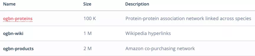
Node prediction

Odbn proteins: protein data set, which has an association network between proteins and includes a variety of organisms;
Odbn Wiki: the network formed by Wikipedia data;
Ogbn products: a network of products that Amazon customers buy at the same time.

The data set currently included in the benchmark.

From the type of data set, it covers several existing fields that need graph representation learning: Biology / molecular chemistry, natural language processing, commodity recommendation system network, etc. In addition, the amount of these graph data is also very large. For example, the data volume of ogbn wiki has reached the level of one million (nodes), and the smallest ogbn proteins has 100K. This is larger than many previous graph data, so it can better evaluate the performance of the model.

Connection prediction

There are more data sets in connection prediction, including:

Ogbi DDI: drug interaction network;
Ogbi Biomed: Atlas of human biomedical knowledge;
Ogbi PPA: relationship network between proteins;
Ogbi reviews: Amazon's user product review data set;
Ogbi citations: Microsoft academic citation network atlas.

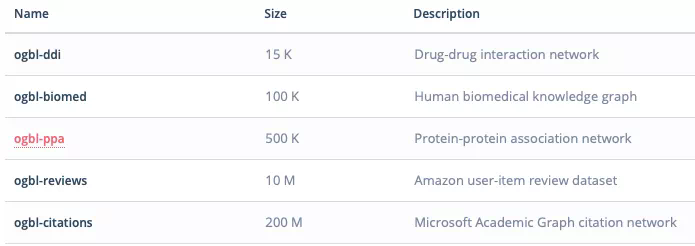
Compared with node data sets, connection prediction data sets are more and more diverse.

Figure prediction

OGB also provides task data sets for predicting graphs, including:

Ogbg mol: molecular prediction, from MoleculeNet;
Syntax of BG code segment tree;
Ogbg PPI: interaction network between proteins;

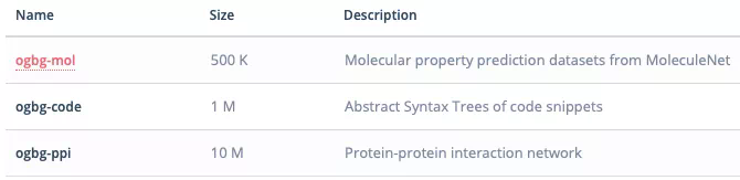
On the whole, there are many data sets biased towards medicine and biology. Professor Zhang Zheng believes that there may be two reasons for this. First, Jure, the project leader, has done a lot of work in this field, so it is natural to promote the open source of these data sets. Another reason is that the map data of drug molecules is relatively clean and less noise. The structure of drugs is 3D, which may require more complex and deeper layers of models to solve relevant problems.

For what data sets will be added in the future, Professor Zhang believes that there is not enough data about heterogeneous graphs, and many data in reality are represented by heterogeneous graphs. However, the role of OGB is still obvious. It can well improve the ability of open source graph neural network framework and promote the open source community to focus on solving practical problems.

In addition, the OGB data set lacks data sets in finance, credit investigation and other fields, especially anti fraud. This may be due to the loss of too many features after desensitization of anti fraud data sets, but the shortcomings are not hidden. OGB undoubtedly helped graph neural network break away from the so-called "toy model" stage and gradually enter industrial application.

Data loading and evaluation

OGB needs special code to extract such a huge amount of data. It is reported that all open source data sets can be extracted and loaded with specific code, using the data in the process and in-depth learning framework_ Loaders are similar. However, before using it, we need to simply use "pip install ogb" to complete the installation. At present, OGB library mainly depends on common modeling libraries such as PyTorch, NumPy and scikit learn. Of course, graph neural network library can also choose DGL or PyTorch geometry freely.

DGL: https://github.com/dmlc/dgl

PyG: https://github.com/rusty1s/pytorch_geometric

Now take node prediction as an example. OGB supports both PYG and DGL diagrams to represent the data loading method in the learning framework. The loading code is as follows:

1. PYG

from ogb.nodeproppred.dataset_pyg import PygNodePropPredDataset
dataset = PygNodePropPredDataset(name = d_name) num_tasks = dataset.num_tasks # obtaining number of prediction tasks in a dataset
splitted_idx = dataset.get_idx_split()train_idx, valid_idx, test_idx = splitted_idx["train"], splitted_idx["valid"], splitted_idx["test"]graph = dataset[0] # pyg graph object

2. DGL

from ogb.nodeproppred.dataset_dgl import DglNodePropPredDataset
dataset = DglNodePropPredDataset(name = d_name)num_tasks = dataset.num_tasks # obtaining number of prediction tasks in a dataset
splitted_idx = dataset.get_idx_split()train_idx, valid_idx, test_idx = splitted_idx["train"], splitted_idx["valid"], splitted_idx["test"]graph, label = dataset[0] # graph: dgl graph object, label: torch tensor of shape (num_nodes, num_tasks)

It can be seen that the code is very simple and easy to use. Where "d_name" can be replaced with the name of any data set.

At the same time, the project provides some sample code to evaluate each data set. As follows:

from ogb.nodeproppred import Evaluator
evaluator = Evaluator(name = d_name) print(evaluator.expected_input_format) print(evaluator.expected_output_format)

Here, the user can understand the specific format of input and output for this data set.

Then, the user can pass the input dictionary into the evaluator to understand the actual performance:

# In most cases, input_dict is# input_dict = {"y_true": y_true, "y_pred": y_pred} result_dict = evaluator.eval(input_dict)

It is reported that OGB officials have indicated that the open source framework DGL dominated by Shanghai AWS AI research institute is one of the platforms for data import. At present, DGL is compatible with PyTorch and MxNet as back-end engines, and TensorFlow is also under development. In fact, DGL has been working on heterogeneous graph and scalability for a long time, so the next step may be to combine new technologies with OGB in related fields to promote the development of open source framework.

Zhang Zheng said, "DGL now has a model base with good results in the pharmaceutical field. With OGB data set, the model base can be iterated, and then it should be further improved."

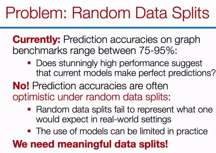
Why is segmenting graph data a problem?

In Jure Leskovec's speech, he specially emphasized the data segmentation method adopted by OGB, which can build a more reasonable evaluation scheme. He said that it seems that random data segmentation is not a matter of concern, but when we randomly divide the data into training, verification and test sets, it is likely that the prediction accuracy looks very good. But in fact, the effect of random segmentation model verification is too overestimated.

Jure Leskovec cited an example. For example, natural science researchers, the data they collect every time is certainly not repeated. They need to do a series of new experiments every time, so the model is making predictions outside the distribution every time. This requires that the data segmentation method should be very reasonable, and the generalization ability of the model should be strong enough to deal with the data prediction outside the distribution.

Turning to the issue of data segmentation, Professor Zhang Zheng said: "when we discussed with researchers in the pharmaceutical industry, we were reminded that it is not advisable to do random segmentation on the training set, because the molecular graph samples have structural properties, and the assumption of independent and identically distributed will affect the generalization ability of the model. I think there are the same problems in other fields."

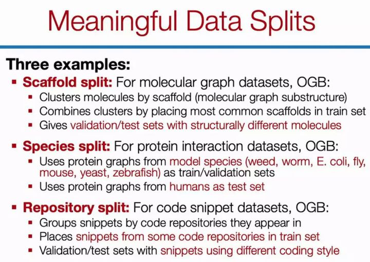
In order to deal with this situation, the data segmentation method adopted by OGB is also very interesting. For example, for molecular graph data sets, the segmentation method can be molecular scaffold. Specifically, we can cluster through the molecular substructure, and then take the commonly used clusters as the training set and other unusual clusters as the verification and test set. This processing method will force the neural network to obtain higher generalization, otherwise it can not predict those molecules with different substructures.

The same is true for species segmentation or code base segmentation. In essence, these data segmentation attempts to move a small part out as a whole for testing.

Finally, Jure Leskovec also showed that they expected OGB to be not only a widely used research resource, but also a real test environment for various new tasks or new models. In the near future, OGB will further support more graph datasets and more graph modeling tasks, and provide an open LeadBoard at the same time. With such LeadBoard, we can more intuitively evaluate the characteristics of various graph neural networks and understand which case their effect is the best.

Keywords: Machine Learning AI neural networks

Added by scopley on Wed, 09 Mar 2022 09:47:27 +0200

Programming VIP