The picture comes from the Internet. If there is infringement, contact to delete it.
This study is divided into two parts. The first part is the video learning part, and the second part is the code learning part.
Part1 video learning
Video 1 Introduction
one ️⃣ Turing test
Judge whether the box is a person or a machine outside the black box.
Ex: verification code system.
2️⃣ GAN
In World War II, the Allies cracked Germany's Enigma system by simulating the process of Enigma password generation. This idea is reflected in today's adversarial generation network (GAN).
Keywords: deep learning model, unsupervised learning, (at least) two modules (Generative Model and discriminant model))
In the original GAN theory, G and D are not required to be neural networks, but only functions that can fit the corresponding generation and discrimination. However, in practice, deep neural network is generally used as G and D.
Discriminant model: given a picture, judge whether the animal in the picture is a cat or a dog
Generation model: generate a new cat (not in the data set) from a series of cat pictures
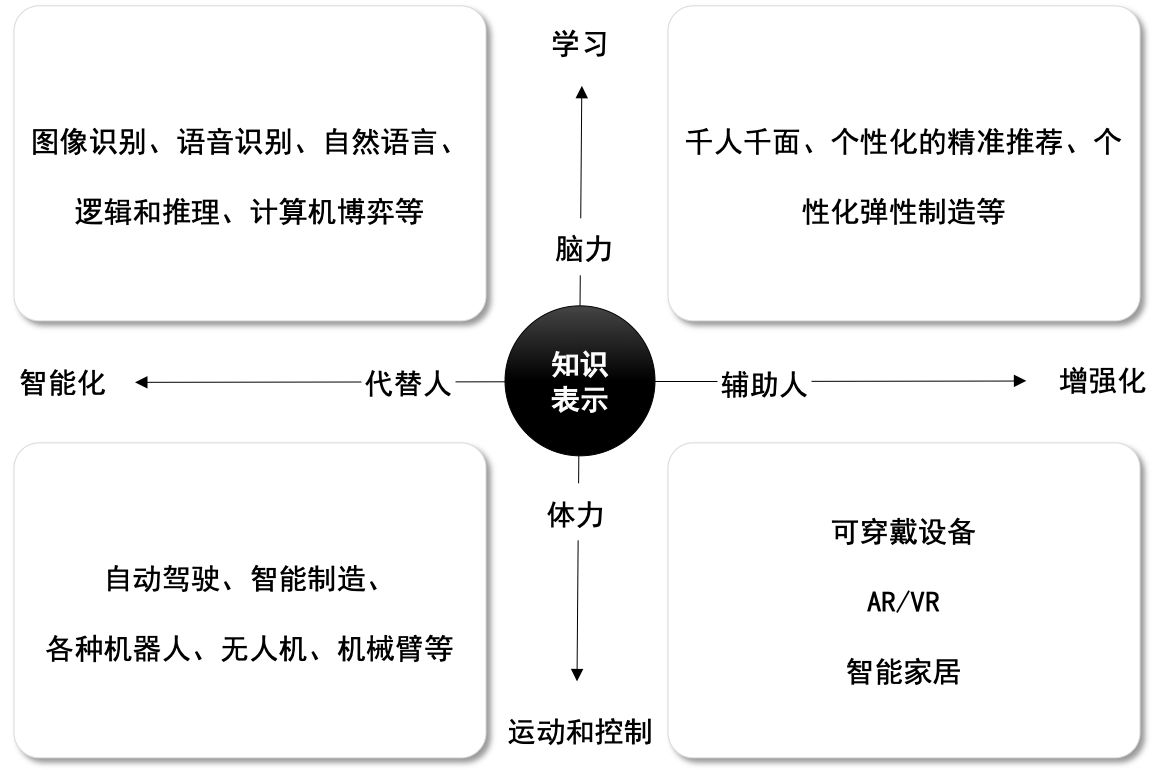
three ️⃣ Three levels of artificial intelligence
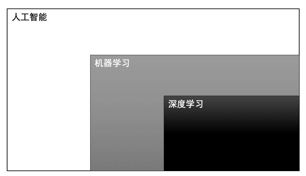
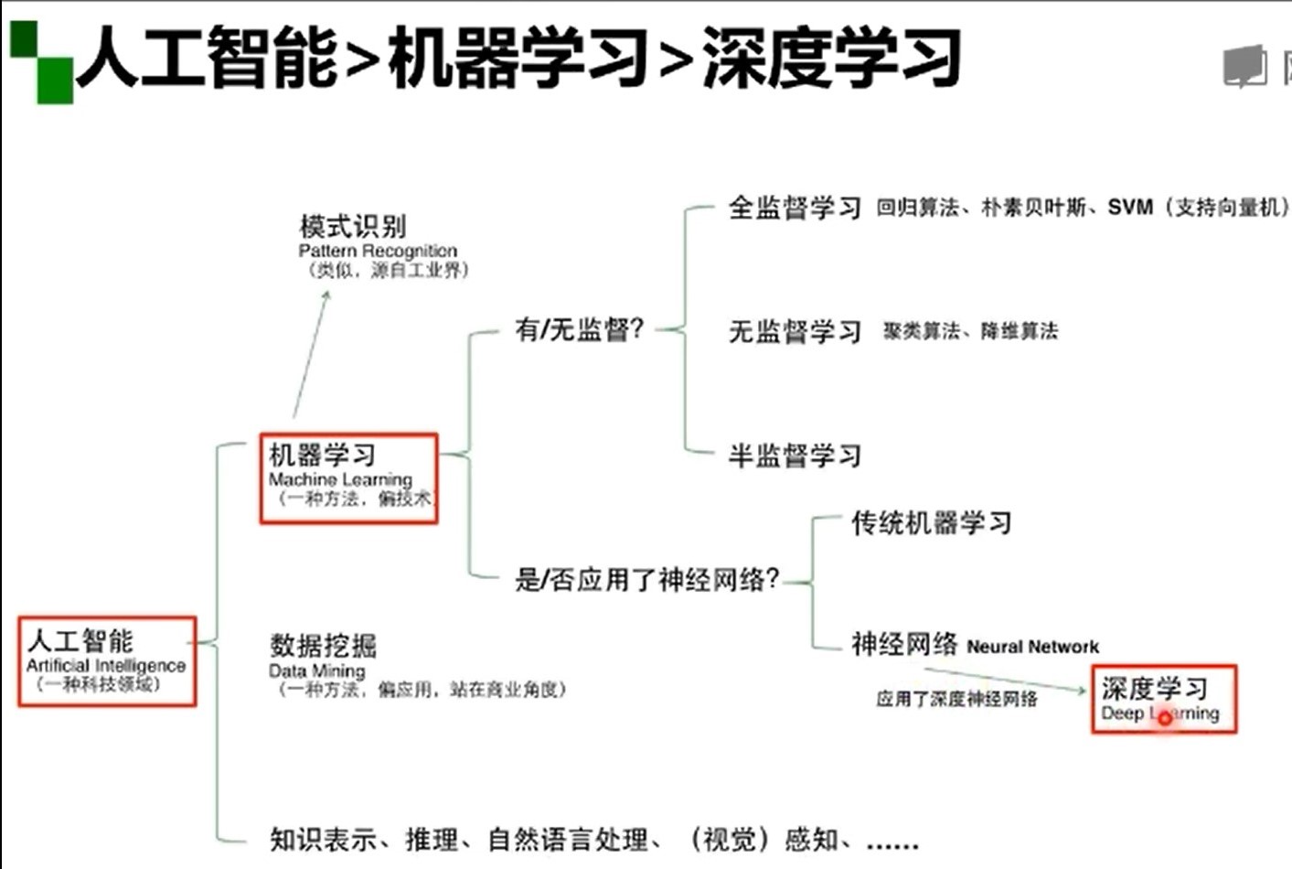
four ️⃣ AI > Machine Learning > deep learning
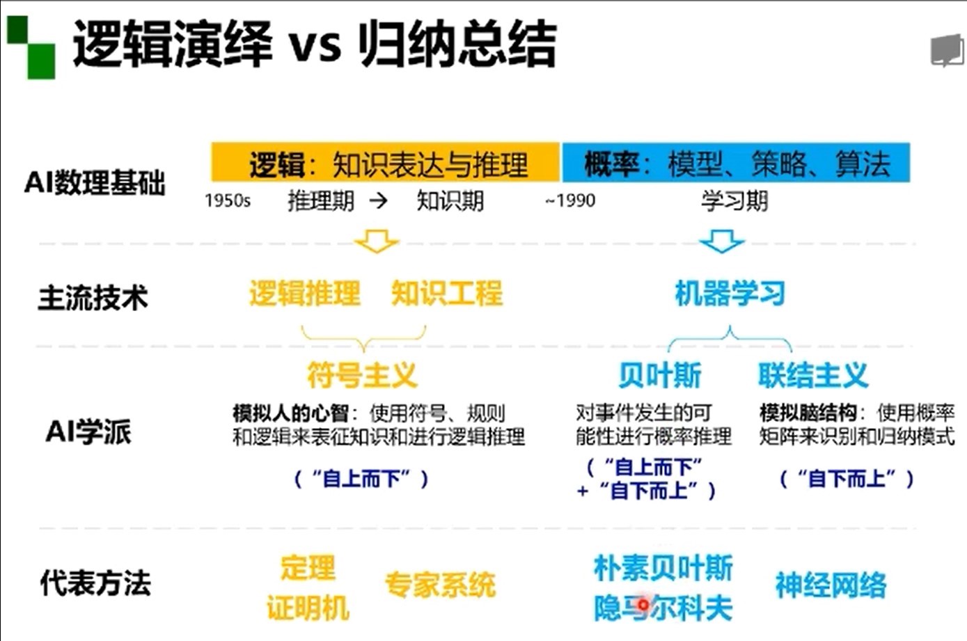
five ️⃣ Logical deduction and induction
six ️⃣ machine learning
keywords: find an approximate solution.
In practical applications, features are often more important than classifiers.
- Model, strategy and method.
Model (assumptions about the problem mapping to be learned)
According to the existing data set, we know the relationship between input and output results. According to this known relationship, an optimal model is trained.
What is supervised, unsupervised and intensive learning?
Parameters refer to the parameters of data distribution. The parametric model can make assumptions about the data distribution in advance.
The generation model models the joint distribution of inputs and outputs
Discriminant model models the conditional distribution of output under input conditions
- Common methods of machine learning

- Manual design features
Feature extraction: extract some effective features from the original data.
Feature transformation: process features to a certain extent, such as dimension increase and dimension reduction.
Feature extraction: PCA, LDA
Feature selection: mutual information, TF-IDF
- Traditional machine learning and deep learning
A.Rule-based systems
Hand-designed program
B.Classic machine learning
Hand-designed feature
Mapping from features
C.Simple representation learning
Features
Mapping from features
D.Deep learning
Simple features
More complex features
Mapping from features
From top to bottom, the role of people is weakened and the ability of machine autonomous learning is enhanced.
Video 2 overview of deep learning
one ️⃣ "Can't" of deep learning
1. The algorithm output is unstable and easy to be "attacked"
Ex: change a pixel value against the sample.
2. The model has high complexity and is difficult to correct and debug
3. The model level is highly complex and the parameters are opaque
Ex: Inception (GoogLeNet), residual, door structure
Inception

Residual (ResNet)

4. The end-to-end training method has strong dependence on data and poor model increment
T
e
s
t
l
o
s
s
−
T
r
a
i
n
i
n
g
l
o
s
s
≤
N
m
Test loss - Training loss ≤ \sqrt{\frac{N}{m}}
Testloss−Trainingloss≤mN
m: Training sample
N: Model effective capacity
5. Focus on intuitive perception problems and do nothing about open reasoning problems
6. Human beings cannot effectively introduce and supervise, and machine bias is difficult to avoid
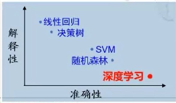
two ️⃣ Interpretability and generalization
 three ️⃣ M-P neuron
y = f(
∑
1
n
\sum_1^n
∑1nwixi -
Θ
\Theta
Θ)
four ️⃣ Activation function
1. Linear function (Ex: identity function)
2. Slope function
3. Threshold function (Ex: step function)
4. Symbolic function
five ️⃣ Sigmoid function
y(x) =
1
1
+
e
<
s
u
p
>
−
x
<
/
s
u
p
>
\frac{1}{1+{e<sup>{-x}</sup>}}
1+e<sup>−x</sup>1
y(x)' = y(x)(1 - y(x))
six ️⃣ Single layer perceptron
I understand that for MP neurons that can learn, the parameter w is not preset.
six ️⃣ Multilayer perceptron
With multiple neuronal layers
Perceptron with multiple hidden layers
seven ️⃣ Universal approximation theorem
If a hidden layer contains enough neurons, the three-layer feedforward neural network (input hidden layer output) can approach any predetermined continuous function with any accuracy.
y = a(W * x + b)
Complete input - > output space transformation
W * x: dimension increase / dimension decrease; Zoom in / out; rotate
+b: Translation
a(·): bending
Deeper and wider do not necessarily enhance the effect.
eight ️⃣ Gradient disappearance
After continuous derivation, the value of each derivative is very small, resulting in the final result close to 0.
nine ️⃣ Error back propagation
F(x) = fn(fn-1...f2(f(x) *
Θ
\Theta
Θ1 + b) *
Θ
\Theta
Θ2 +b)...)
Compare the difference between the actual result and the final result. The difference is to reduce the weight; Otherwise, increase the weight.
It can be adjusted through Learning Rate
Therefore, BP algorithm is easy to over fit (it performs well in the training set, but not in the new data set). It can be improved by stopping in advance, adjusting parameters with the training set and adjusting errors with the verification set.
Part2 code learning
Basic operations in Python
import torch
x = torch.tensor(666)
print(x)
# one-dimensional
x = torch.tensor([1, 2, 3, 4, 5, 6])
# two-dimensional
# Matrix with two rows and three columns
x = torch.ones(2, 3)
# Arbitrary dimension
x = torch.ones(2,3, 4)
# Create an empty tensor, x rows, y columns

x = torch.empty(x, y)

# Create a randomly initialized tensor

x = torch.rand(5, 3)

# Create a tensor with all zeros, and the data type in it is long
x = torch.zeros(5,3,dtype=torch.long)

# Initialize a new tensor with a known tensor

y = x.new_ones(5,3)

# Redefine the type of the original tensor

z = torch.randn_like(x, dtype = torch.float)

# output

print(m\[0][2])

print(m[:, 1])

# matrix multiplication

m @ v

# Matrix transpose (3 methods)

print(m.t())

print(m.transpose(0, 1))

print(m.permute(1, 0))
Spiral classifciation
import random
import torch
from torch import nn, optim
import math
from IPython import display
from plot_lib import plot_data, plot_model, set_default

# Because colab supports GPU, torch will run on GPU
device = torch.device("cuda:0" if torch.cuda.is_available() else "cpu")
print('device: ', device)

# Initialize random number seed. The parameters of the neural network are randomly initialized,
# Different initialization parameters often lead to different results. When better results are obtained, we usually hope that the results can be reproduced,
# Therefore, in pytorch, this goal can also be achieved by setting random number seeds
seed = 12345
random.seed(seed)
torch.manual_seed(seed)

N = 1000  # Number of samples per type
D = 2  # Characteristic dimension of each sample
C = 3  # Category of samples
H = 100  # Number of hidden layer units in neural network
torch.manual_seed(seed) is used to facilitate reproduction
After setting the random seed, the output result of the file is the same every time you run it
copy all the tensor variables at the beginning of reading data to the GPU specified by device, and the subsequent operations are carried out on the GPU.
Multi GPU
device = torch.device("cuda:0" if torch.cuda.is_available() else "cpu")

model = Model()

if torch.cuda.device_count() > 1:

  model = nn.DataParallel(model,device_ids=[0,1,2])

model.to(device)
To: Code in case of multiple GPU s
X = torch.zeros(N * C, D).to(device)
Y = torch.zeros(N * C, dtype=torch.long).to(device)
for c in range(C):
    index = 0
    t = torch.linspace(0, 1, N) # Take 10000 numbers evenly between [0, 1] and assign them to t
    # The following code need not be understood too much. In short, three types of samples (which can form a spiral) are calculated according to the formula
    # torch.randn(N) is a group of random numbers with N mean values of 0 and variance of 1. Pay attention to distinguish it from rand
    inner_var = torch.linspace( (2*math.pi/C)*c, (2*math.pi/C)*(2+c), N) + torch.randn(N) * 0.2

    # The (x,y) coordinates of each sample are saved in X
    # The categories of samples stored in Y are [0, 1, 2]
    for ix in range(N * c, N * (c + 1)):
        X[ix] = t[index] * torch.FloatTensor((math.sin(inner_var[index]), math.cos(inner_var[index])))
        Y[ix] = c
        index += 1

print("Shapes:")
print("X:", X.size())
print("Y:", Y.size())
torch.linspace(0, 1, N) divides the interval (0, 1) into N shares