What is a graph
In the previous article, we learned the concept of tree, focusing on binary tree. Graph is a little similar to tree in topology, but graph is not a tree
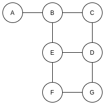
Intuitively, let's first look at the topology of a graph:
Undirected graph
The above shows an undirected graph. An undirected graph is a graph without direction. As long as two nodes are connected, they can go from one node to another
We can understand it as a simplified map. A-G represents location
Generally, we have the following general concepts for graphs:
- The nodes of a graph are called vertices;
- The connection between vertices (nodes) is called edge;
- How many edges a vertex (node) has is called the degree of the vertex (node);
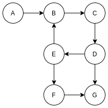
Correspondingly, there is also a directed graph. A directed graph is a directed graph. The edges of two linked vertices have directions and can go from one vertex to another. If the two vertices are interconnected, there must be at least two edges in different directions
A directed graph is similar to a one-way traffic lane
Directed graph
The edges of a directed graph may point from a vertex or point to a vertex. We call the number of edges pointed from the vertex the degree of the vertex, and the number of edges pointing to a vertex the degree of the vertex
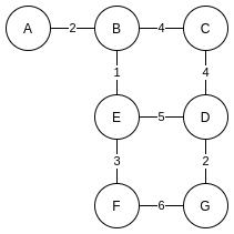
Compared with a map, the edge between two vertices can not only represent the connection relationship, but also the distance. Each edge is given a "distance" parameter (weight). Such a graph is called a weighted graph:
Weighted graph
Analogical object of graph
This data structure can represent some common objects in daily life. Here are some examples:
- The map can be represented by a graph. The vertex is the place, the edge is the path between two places, and the weight on the edge can represent the distance;
- Friends can also be represented by a graph. The vertex is each individual, the edge indicates whether there is a connection between the two individuals, and the weight on the edge can indicate the degree of favor;
- The compiler also uses graphs. The header file include during C/C + + compilation can be represented by graph vertices, and the directed edges can represent dependencies;
Adjacency table storage method
How are diagrams stored?
It is a very intuitive storage method similar to a tree, and uses a linked list to represent the topology of the graph But the problem with this method is that we don't know how many edges each vertex of the graph will have, so it's not easy to define the structure
The adjacency list storage method also uses the linked list storage method. It represents each vertex as the head of the linked list, and the subsequent node is other vertices connected with the vertex. The following figure shows the adjacency list storage method of undirected graph:
Adjacency table storage method
1 2 3 4 5 | |
Above, val represents the value of the vertex, and link stores other vertices connected with this vertex
The link here looks like sequential storage. If the time complexity is O(n) when searching for another vertex connected to the vertex, we can use the search binary tree or red black tree to replace the sequential structure and improve the search efficiency. The specific data structure needs to be analyzed according to the specific scene
Breadth first search (BFS)
The search / traversal of graphs is similar to that of trees. It should be noted that graphs can have loops and do not fall into dead loops
Breadth first search is to access all the child nodes of the starting node first, and then all the child nodes of the asking child node. From the structure of the tree, it is a layer by layer access
Let's use the tree structure to show how BFS Searches:
BFS
Define the structure of the diagram first:
1 2 3 4 5 6 7 8 | |
};
using Map = Graph<char>;
Our main function uses the undirected graph above:
1 2 3 4 5 6 7 8 9 10 11 12 13 14 15 16 | |
}
link_ The first element of the bar element of map represents a vertex, and the subsequent elements represent other vertices connected to the vertex;
Write a graph printing function to output graphs using adjacency table storage method:
1 2 3 4 5 6 7 8 9 10 11 12 13 | |
Convert the initialization data of the graph into adjacency table storage:
1 2 3 4 5 6 7 8 9 10 11 12 13 14 15 16 17 18 19 20 21 22 23 24 25 26 27 28 29 30 31 32 | |
}
After initializing the graph, we get the output:
1 2 3 4 5 6 7 | A(0x11852a0)->B(0x11852c0) B(0x11852c0)->A(0x11852a0)->C(0x11852e0)->E(0x1185320) C(0x11852e0)->B(0x11852c0)->D(0x1185300) D(0x1185300)->C(0x11852e0)->E(0x1185320)->G(0x1185360) E(0x1185320)->B(0x11852c0)->D(0x1185300)->F(0x1185340) F(0x1185340)->E(0x1185320)->G(0x1185360) G(0x1185360)->D(0x1185300)->F(0x1185340) |
For the breadth first search algorithm, we use the open-close table
- The open table stores the nodes to be accessed next. Generally, a double ended queue can be used;
- The close d table stores the accessed nodes. Generally, any container can be used;
Next, determine the operation for each node:
- Judge whether the node has been accessed (whether it is in the close table):
1 2 3 4 5 6 7 8 | |
- Put the nodes to be accessed next into the open table:
1 2 3 | |
- Take the node from the open table and access:
1 2 3 4 5 | |
Attention should be paid to the operation of the open table. When pushing, the node is pushed to the end, and when taking elements, it is taken from the beginning
- For node processing, cout is used here for simplicity
1 2 3 | |
With the above basic operations, breadth first traversal is implemented as follows:
1 2 3 4 5 6 7 8 9 10 11 12 13 14 15 16 17 18 19 20 21 22 23 24 25 26 27 28 29 30 31 32 33 34 35 36 37 38 39 40 41 42 43 44 | |
}
Output:
Depth first search (DFS)
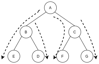
From the tree structure, depth first search is accessed from the root node to the leaf node
Let's use the tree structure to show how DFS Searches:
DFS
The logic of depth first search is basically the same as that of breadth first search. The difference lies in the different ways of obtaining values from the open table
In breadth first search, we push the node to be accessed to the end of the open table, and then take the next accessed node from the header of the open table. As a result, we first access all the child nodes of the node, and then access all the child nodes of the child node
Depth first search is to push the node to be accessed to the end of the open table, and then take the next accessed node from the end of the open table. This is equivalent to tracing the child nodes from a few points to the end
The following is the openGet operation in depth first search:
1 2 3 4 5 | |
The complete implementation is as follows:
1 2 3 4 5 6 7 8 9 10 11 12 13 14 15 16 17 18 19 20 21 22 23 24 25 26 27 28 29 30 31 32 33 34 35 36 37 38 39 40 41 42 43 44 45 46 | |
}
Output:


