Graph of Data Structure
1. introduction
Graph structure is also a kind of non-linear data structure. There are many examples of graph structure in life, such as communication network, traffic network, interpersonal network and so on, which can be reduced to graph structure. Each node of the graph structure can be related to each other, which is more complex than the tree structure.
The following figure is a simple graph structure:

2. Relevant concepts
1. digraph
2. undirected graph
3. Degree of a vertex: The number of edges connecting a vertex is called the degree of the vertex. Directed graphs are divided into degrees of entry and degrees of exit.
4. Adjacent vertices: Two vertices of an edge. Directed graphs can be divided into two types: inbound adjacent vertices and outbound adjacent vertices.
5. undirected complete graph: there is an edge between two vertices.
6. Directed complete graph: There are two opposite sides between each vertex. For a directed complete graph with N nodes, the number of edges is N(N-1), twice that of undirected complete graph.
7. Subgraphs: Like subsets, vertices and edges of subgraphs are primitive.
-
8. Path: There may be more than one line between two vertices, each of which may be different in length. The path can be divided into three forms:
- Simple path: vertices on a path do not appear repeatedly;
- Ring: The first vertex of a path is the same as the last vertex. It is called a ring, sometimes in a loop.
- Simple loop: The first vertex of the path is the same as the last vertex, and the other vertices that do not repeat are called simple loop.
-
9. Connected, connected graphs and connected components:
- If there is a path between two vertices, then the two vertices are connected.
- Any two vertices in an undirected graph are connected, which is called a connected graph.
- Maximally connected subgraphs in undirected graphs are called connected components.
The connected component of a connected graph has and only has one, which is itself.
-
10. Strongly connected graphs and strongly connected components:
- If there is a path between the two vertices, then the two vertices are connected. Note that because of orientation, sometimes it may be that Vi-> Vj is connected and Vj-> Vi is not connected.
- If any two vertices in a digraph are connected, then they are strongly connected.
- The maximum strongly connected subgraph of a digraph is called the strongly connected component of the graph.
The strong connected component of a strongly connected graph has one and only one component, which is itself.
11. Weight: The value represented on the edge, which is the weight of the edge. Adding weights to undirected graphs is called undirected weighted graphs, and adding weights to digraphs is called directed weighted graphs. Right in life can indicate the length of the road in the traffic map, intimacy in interpersonal relationships and so on.
12. network: Another name for a graph with weights on its edges, which is more appropriate for practical applications.
3. Storage of Graphs
In practical applications, we usually use arrays to save vertex information separately, and then use two-dimensional arrays to preserve the relationship between vertices. This array that preserves the relationship between vertices is called an adjacency matrix.
char[] Vertex = new char[MaxNum];  //Save vertex information
int[][] EdgeWeight = new int[MaxNum][MaxNum];  //Save edge
The edges of this undirected graph can be represented as follows
Vertex[0] = 1;
Vertex[1] = 2;
Vertex[2] = 3;
Vertex[3] = 4;
Vertex[5] = 5;
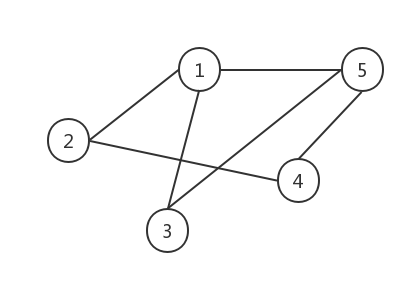
EdgeWeight two-dimensional arrays are used to represent edges. If there are edges, 1 will be saved, and if there are no edges, 0 will be saved. For example, tables between 1 and 2 can be expressed as:
//The bottom corner of an array starts at 0.
EdgeWeight[0][1] = 1;
EdgeWeight[1][0] = 1;
The adjacency matrix of this graph:
| 0 | 1 | 1 | 0 | 1 |
|---|---|---|---|---|
| 1 | 0 | 0 | 1 | 0 |
| 1 | 0 | 0 | 0 | 1 |
| 0 | 1 | 0 | 0 | 1 |
| 1 | 0 | 1 | 1 | 0 |
Because it is an undirected graph, it is symmetrical on the lower left and right, but not on the digraph.
4. Code examples
Next, we use a code example to look at the tree structure initialization, emptying and output traversal operations:
package com.wangjun.datastructure;

public class GraphTest {
    private final int MaxNum = 5; // max vertex

    public static void main(String[] args) {
        GraphTest gt = new GraphTest();
        GraphMatrix gm = gt.new GraphMatrix();
        gt.createGraph(gm);
        gt.outGraph(gm);
        gt.deepTraGraph(gm);
    }


    // Define adjacency matrix structure
    class GraphMatrix {
        char[] Vertex = new char[MaxNum]; // Save vertex information, numbers or letters
        int GType; // Type, 0: undirected graph, 1: digraph
        int vertexNum; // Number of vertices
        int EdgeNum; // Number of edges
        int[][] EdgeWeight = new int[MaxNum][MaxNum]; // Right to Preserve Edges
        int[] isTrav = new int[MaxNum]; // Traversal flag
    }

    // Creating Adjacency Matrix Graph
    // Here we create a graph that manually creates a 5-node map, corresponding to the graph above.
    public void createGraph(GraphMatrix gm) {
        gm.Vertex[0] = '1';
        gm.Vertex[1] = '2';
        gm.Vertex[2] = '3';
        gm.Vertex[3] = '4';
        gm.Vertex[4] = '5';

        gm.GType = 0;
        gm.vertexNum = 5;
        gm.EdgeNum = 6;
        gm.EdgeWeight[0][1] = 1;
        gm.EdgeWeight[1][0] = 1;
        gm.EdgeWeight[0][2] = 1;
        gm.EdgeWeight[2][0] = 1;
        gm.EdgeWeight[0][4] = 1;
        gm.EdgeWeight[4][0] = 1;
        gm.EdgeWeight[2][4] = 1;
        gm.EdgeWeight[4][2] = 1;
        gm.EdgeWeight[1][3] = 1;
        gm.EdgeWeight[3][1] = 1;
        gm.EdgeWeight[3][4] = 1;
        gm.EdgeWeight[4][3] = 1;
    }

    // Empty map
    public void clearGraph(GraphMatrix gm) {
        for (int i = 0; i < MaxNum; i++) {
            for (int j = 0; i < MaxNum; j++) {
                gm.EdgeWeight[i][j] = 0;
            }
        }
    }

    // Display graph, that is, display adjacency matrix
    public void outGraph(GraphMatrix gm) {
        // Output vertex information
        System.out.println("Vertex:");
        for (int i = 0; i < MaxNum; i++) {
            System.out.print(gm.Vertex[i] + "  ");
        }
        System.out.println();
        // Output side Information
        System.out.println("Edge:");
        for (int i = 0; i < MaxNum; i++) {
            for (int j = 0; j < MaxNum; j++) {
                System.out.print(gm.EdgeWeight[i][j] + "  ");
            }
            System.out.println();
        }
    }

    /*
     * Traversal graphs, which access vertices one by one, use isTrav arrays to indicate whether the node has been traversed
     * Generally used ergodic graph methods: breadth-first ergodic method and depth-first ergodic method. This function takes depth-first ergodic method as an example.
     * The depth traversal method is similar to the tree's precedent traversal. The specific execution process is as follows:
     * 1)Select an unaccounted vertex Vi from the isTrav array and mark it as 1 to indicate that it has been visited
     * 2)Depth-first traversal from an untried adjacent point of Vi
     * 3)Repeat step 2 until all vertices in the graph that are path-wise to Vi have been accessed
     * 4)Repeat steps 1) to 3 until all vertices in the graph have been accessed
     * Depth-first traversal is a recursive process
     */
    public void deepTraGraph(GraphMatrix gm) {
        // Clear vertex access flag
        for (int i = 0; i < gm.vertexNum; i++) {
            gm.isTrav[i] = 0;
        }
        System.out.println("Depth-first traversal node:");
        for (int i = 0; i < gm.vertexNum; i++) {
            // If the node is not traversed
            if (gm.isTrav[i] == 0) {
                deepTraOne(gm, i);// Call function traversal
            }
        }
    }

    //Execution function of depth traversal
    public void deepTraOne(GraphMatrix gm, int n) {
        // Beginning with the nth node, the depth traversal graph
        gm.isTrav[n] = 1;
        // Output node data
        System.out.println("node:" + gm.Vertex[n] + "  ");

        // Adding operations to process nodes
        for (int i = 0; i < gm.vertexNum; i++) {
            if (gm.EdgeWeight[n][i] != 0 && gm.isTrav[i] == 0) {
                deepTraOne(gm, i);// Recursive traversal
            }
        }
    }

}