Pandas is the most widely used data analysis and operation Library in Python. It provides many functions and methods to speed up the "data analysis" and "preprocessing" steps.

In order to better learn Python, I will take the customer churn data set as an example to share "30" functions and methods most commonly used in data analysis. The data "text" can be downloaded.

The data are as follows:

import numpy as np
import pandas as pd
df = pd.read_csv("Churn_Modelling.csv")
print(df.shape)
df.columns

Result output

(10000, 14)
Index(['RowNumber', 'CustomerId', 'Surname', 'CreditScore', 'Geography','Gender', 'Age', 'Tenure', 'Balance', 'NumOfProducts', 'HasCrCard','IsActiveMember', 'EstimatedSalary', 'Exited'],dtype='object')

1. Delete column

df.drop(['RowNumber', 'CustomerId', 'Surname', 'CreditScore'], axis=1, inplace=True)
print(df[:2])
print(df.shape)

Result output

  Geography  Gender  Age  Tenure  Balance  NumOfProducts  HasCrCard  \
0    France  Female   42       2      0.0              1          1   

   IsActiveMember  EstimatedSalary  Exited  
0               1        101348.88       1  
(10000, 10)

Description: set the axis parameter to 1 to place columns and 0 to rows. Set the inplace=True parameter to True to save the changes. We have reduced the number of columns from 14 to 10.

2. Select a specific column

We read some column data from the csv file. You can use the usecols parameter.

df_spec = pd.read_csv("Churn_Modelling.csv", usecols=['Gender', 'Age', 'Tenure', 'Balance'])
df_spec.head()

3.nrows

You can use the nrows parameter to create a data frame containing the first 5000 lines of the csv file. You can also use the skirows parameter to select rows from the end of the file. Skirows = 5000 means that we will skip the first 5000 lines when reading csv files.

df_partial = pd.read_csv("Churn_Modelling.csv", nrows=5000)
print(df_partial.shape)

4. Sample

After creating the data frame, we may need a small sample to test the data. We can use n or frac parameters to determine the sample size.

df= pd.read_csv("Churn_Modelling.csv", usecols=['Gender', 'Age', 'Tenure', 'Balance'])
df_sample = df.sample(n=1000)
df_sample2 = df.sample(frac=0.1)

5. Check the missing value

The isna function determines the missing value in the data frame. By using isna with the sum function, we can see the number of missing values in each column.

df.isna().sum()

6. Add missing values using loc and iloc

Add missing values using loc and iloc. The differences are as follows:

• loc: select labeled
• iloc: select index

We first create 20 random indexes for selection

missing_index = np.random.randint(10000, size=20)

We will use loc to change some values to NP Nan (missing value).

df.loc[missing_index, ['Balance','Geography']] = np.nan

20 values are missing in the Balance and Geography columns. Let's use iloc as another example.

df.iloc[missing_index, -1] = np.nan

7. Fill in missing values

The fillna function is used to fill in missing values. It provides many options. We can use a specific value, an aggregate function (such as the mean), or the previous or next value.

avg = df['Balance'].mean()
df['Balance'].fillna(value=avg, inplace=True)

The method parameter of the fillna function can be used to populate missing values based on the previous or next value in the column (for example, method = "fill"). It can be very useful for sequential data, such as time series.

8. Delete missing values

Another way to handle missing values is to delete them. The following code will delete rows with any missing values.

df.dropna(axis=0, how='any', inplace=True)

9. Select rows according to criteria

In some cases, we need observations (i.e. lines) suitable for certain conditions

france_churn = df[(df.Geography == 'France') & (df.Exited == 1)]
france_churn.Geography.value_counts()

10. Use query to describe conditions

Query functions provide a more flexible way to pass conditions. We can describe them in strings.

df2 = df.query('80000 < Balance < 100000')
#Let's confirm the results by drawing a histogram of the balanced column.
df2['Balance'].plot(kind='hist', figsize=(8,5))

11. Describe the conditions with isin

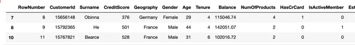
The condition may have multiple values. In this case, it is better to use the isin method rather than writing values alone.

df[df['Tenure'].isin([4,6,9,10])][:3]

12.Groupby function

The Pandas Groupby function is a versatile and easy-to-use function that helps get an overview of the data. It makes it easier to browse data sets and reveal the basic relationships between variables.

We will do several examples of group ratio functions. Let's start with simplicity. The following code will group the rows based on the combination of Geography and Gender, and then give the average churn rate of each group.

df[['Geography','Gender','Exited']].groupby(['Geography','Gender']).mean()

13. Combination of groupby and aggregate function

The agg function allows multiple aggregate functions to be applied on a group, and a list of functions is passed as parameters.

df[['Geography','Gender','Exited']].groupby(['Geography','Gender']).agg(['mean','count'])

14. Apply different aggregation functions to different groups

df_summary = df[['Geography','Exited','Balance']].groupby('Geography').agg({'Exited':'sum', 'Balance':'mean'})
df_summary.rename(columns={'Exited':'# of churned customers', 'Balance':'Average Balance of Customers'},inplace=True)

In addition, the NamedAgg function allows you to rename columns in an aggregate

import pandas as pd
df_summary = df[['Geography','Exited','Balance']].groupby('Geography').agg(Number_of_churned_customers = pd.NamedAgg('Exited', 'sum'),Average_balance_of_customers = pd.NamedAgg('Balance', 'mean'))
print(df_summary)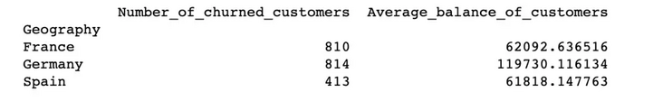

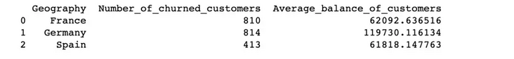
15. Reset index

Have you noticed the data format in the figure above. We can change it by resetting the index.

print(df_summary.reset_index())

16. Reset and delete the original index

In some cases, we need to reset the index and delete the original index at the same time.

df[['Geography','Exited','Balance']].sample(n=6).reset_index(drop=True)

17. Set specific columns as indexes

We can index any column in the data frame.

df_new.set_index('Geography')

18. Insert new column

group = np.random.randint(10, size=6)
df_new['Group'] = group

19.where function

It is used to wrap values in rows or columns based on conditions. The default replacement value is NaN, but we can also specify it as the replacement value.

df_new['Balance'] = df_new['Balance'].where(df_new['Group'] >= 6, 0)

20. Grade function

The rank function assigns a ranking to the value. Let's create a column to rank customers according to their balance.

df_new['rank'] = df_new['Balance'].rank(method='first', ascending=False).astype('int')

21. Number of unique values in the column

It comes in handy when using classification variables. We may need to check the number of unique categories. We can check the size of the sequence returned by the value counting function or use the nunique function.

df.Geography.nunique

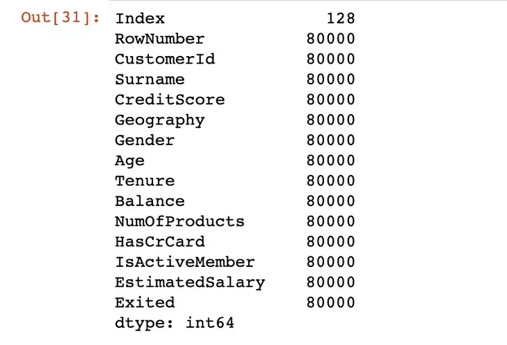
22. Memory usage

Using the function memory_usage, these values show memory in bytes

df.memory_usage()

23. Data type conversion

By default, classification data is stored with the object data type. However, it may lead to unnecessary memory usage, especially when classification variables have a low cardinality.

Low cardinality means that columns have few unique values compared to the number of rows. For example, a geographic column has 3 unique values and 10000 rows.

We can save memory by changing its data type to category.

df['Geography'] = df['Geography'].astype('category')

24. Replacement value

The replace function can be used to replace values in a data frame.

df['Geography'].replace({0:'B1',1:'B2'})

25. Draw histogram

pandas is not a data visualization library, but it makes it very easy to create basic drawings.

I found it easier to create basic drawings using Pandas instead of using other data visualization libraries.

Let's create a histogram of the balanced column.

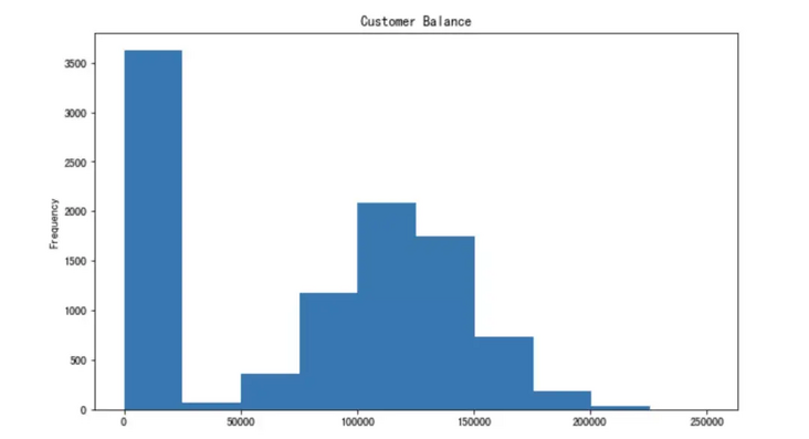
26. Reduce floating point number and decimal point

pandas may display too many decimal points for floating-point numbers. We can easily adjust it.

df['Balance'].plot(kind='hist', figsize=(10,6), 
title='Customer Balance')

27. Change display options

Instead of manually adjusting the display options each time, we can change the default display options for various parameters.

• get_option: returns the current option
• set_option: let's change the display option of the decimal point to 2.

pd.set_option("display.precision", 2)

Some other options that may need to be changed include:

• max_colwidth: the maximum number of characters displayed in the column
• max_columns: the maximum number of columns to display
• max_rows: maximum number of rows to display

28. Calculate the percentage change by column

pct_change is used to calculate the percentage change in the value of the sequence. It is useful when calculating the percentage change in a time series or element order array.

ser= pd.Series([2,4,5,6,72,4,6,72])
ser.pct_change()

29. String based filtering

We may need to filter observations (rows) based on text data (such as customer name). I have added df_new name to the data frame.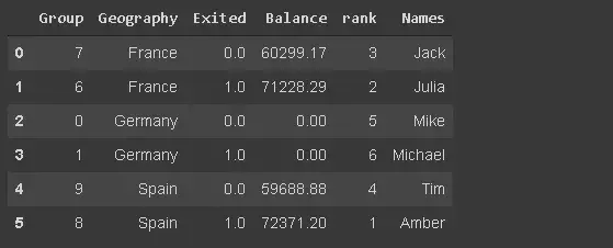

df_new[df_new.Names.str.startswith('Mi')]

30. Set data frame style

We can do this by using the Style property that returns the Style object, which provides many options for formatting and displaying the data frame. For example, we can highlight the minimum or maximum value.

It also allows you to apply custom style functions.

df_new.style.highlight_max(axis=0, color='darkgreen')