catalogue

1. Introduction

2. Detailed explanation of algorithm

2.1 data standardization

2.2} calculate the grey correlation coefficient

2.3 calculation of grey correlation coefficient

3. Case analysis

3.1 reading data

3.2 data standardization

3.3} draw the broken line diagram of x1, x4, X5, X6 and X7

3.4 grey correlation coefficient

Complete code

1. Introduction

For the factors between two systems, the measure of the degree of correlation that changes with time or different objects is called correlation degree. In the process of system development, if the two factors change trend Consistency, i.e. synchronous change degree Higher means that the two are highly related; On the contrary, it is lower. Therefore, the grey correlation analysis method is based on the degree of similarity or difference in the development trend between factors, that is, "grey correlation degree", as a measure of the degree of correlation between factors method.

Grey correlation analysis can be used to measure the degree of correlation of factors, but it is also used in comprehensive evaluation in some papers. Its principle and idea are similar to TOPSIS method.  

2. Detailed explanation of algorithm

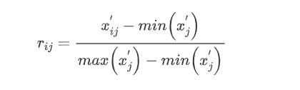
2.1 data standardization

Because the order of magnitude of each indicator is different, it is necessary to compare them within the same range. There are many standardization methods, and only the maximum and minimum standardization method is used here.

Set the standardized data matrix element as rij, and the data matrix element after the index forward is (Xij) '

2.2} calculate the grey correlation coefficient

Our common grey correlation coefficient expression is as follows:

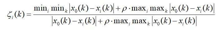
Xo(k) is the reference column and p is the resolution coefficient. Its range is (0 ~ 1), and its function is to control discrimination. The smaller its value is, the greater its discrimination is, and the larger its value is, the smaller its discrimination is. Often take 0.5. At first glance, this formula is still a little difficult to understand. Next, let's introduce its principle in detail.

2.3 calculation of grey correlation coefficient

• Selection of reference vector

For example, study the grey correlation between x2 index and x1 index. Therefore, take column x1 as the reference vector, that is, take who as the reference to study the relationship with whom. Set the reference vector as Y1=x1 and generate a new data matrix X1=x2

• Generate absolute value matrix

Let the generated absolute value matrix be A

A=[X1-Y1], also A=[x2-x1]

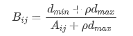
Let dmax be the maximum value of absolute value matrix A and dmin be the minimum value of absolute value matrix A.

• Calculate grey incidence matrix

Let the grey incidence matrix be B

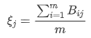
• Calculate grey correlation degree

3. Case analysis

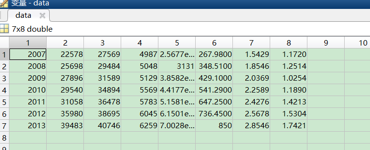
Among them, x1: cargo transportation volume; x2: port cargo throughput; x3: turnover of goods; x4: GDP； x5: fiscal revenue x6: per capita disposable income of urban residents; X7: per capita net income of rural residents. This paper studies the grey correlation between x4-x7 index and x1 index. The data table is as follows:

particular year	x1	x2	x3	x4	x5	x6	x7
2007	22578	27569	4987	2567.7	267.98	1.5429	1.172
2008	25698	29484	5048	3131	348.51	1.8546	1.2514
2009	27896	31589	5129	3858.2	429.1	2.0369	1.0254
2010	29540	34894	5569	4417.7	541.29	2.2589	1.189
2011	31058	36478	5783	5158.1	647.25	2.4276	1.4213
2012	35980	38695	6045	6150.1	736.45	2.5678	1.5304
2013	39483	40746	6259	7002.8	850	2.8546	1.7421

3.1 reading data

data=xlsread('D:\desktop\huiseguanlian.xlsx')

return:

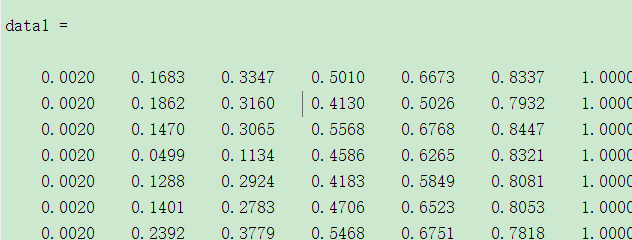
3.2 data standardization

%Data standardization
data1=mapminmax(data',0.002,1) %Normalize to 0.002-1 section

Return:

3.3} draw the broken line diagram of x1, x4, X5, X6 and X7

figure(1)
t=[2007:2013];
plot(t,data1(:,1),'LineWidth',2)
hold on 
for i=1:4
    plot(t,data1(:,3+i),'--')
    hold on
end
xlabel('year')
legend('x1','x4','x5','x6','x7')
title('Grey correlation analysis')

return:

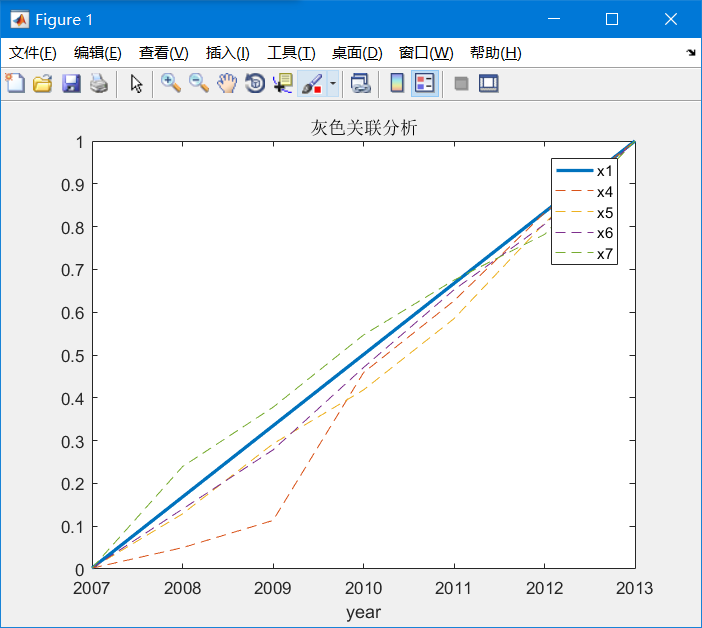
As can be seen from the figure, the trends of these indicators are roughly the same

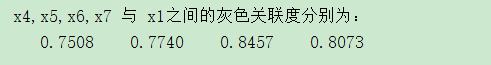
3.4 calculation of grey correlation coefficient

3.4.1 ， get the absolute value of other columns equal to the reference column

%Get the absolute value of other columns equal to the reference column
for i=4:7
    data1(:,i)=abs(data1(:,i)-data1(:,1));
end

3.4.2} get the global maximum and minimum of the absolute value matrix

%The global maximum and minimum of the absolute value matrix are obtained
data2=data1(:,4:7);
d_max=max(max(data2));
d_min=min(min(data2));

3.4.3 definition of resolution coefficient

a=0.5

3.4.4 calculation of grey incidence matrix

data3=(d_min+a*d_max)./(data2+a*d_max);
xishu=mean(data3);
disp(' x4,x5,x6,x7 And x1 The grey correlation degrees between them are:')
disp(xishu)

return:

Complete code

clc;clear;
%Read data
data=xlsread('D:\desktop\huiseguanlian.xlsx');
%Data standardization
data1=mapminmax(data',0.002,1); %Normalize to 0.002-1 section
data1=data1';
%%draw x1,x4,x5,x6,x7 Line chart of
figure(1)
t=[2007:2013];
plot(t,data1(:,1),'LineWidth',2)
hold on 
for i=1:4
    plot(t,data1(:,3+i),'--')
    hold on
end
xlabel('year')
legend('x1','x4','x5','x6','x7')
title('Grey correlation analysis')

%%Calculate grey correlation coefficient
%Get the absolute value of other columns equal to the reference column
for i=4:7
    data1(:,i)=abs(data1(:,i)-data1(:,1));
end

%The global maximum and minimum of the absolute value matrix are obtained
data2=data1(:,4:7);
d_max=max(max(data2));
d_min=min(min(data2));
%Grey incidence matrix
a=0.5;   %Resolution coefficient
data3=(d_min+a*d_max)./(data2+a*d_max);
xishu=mean(data3);
disp(' x4,x5,x6,x7 And x1 The grey correlation degrees between them are:')
disp(xishu)