1. Introduction to OLAP
1. Concepts
OLAP is the abbreviation for On-Line Analytical Processing in English, meaning Online Analytical Processing.This concept was first proposed by E.F.Codd, the father of relational databases, in 1993.OLAP allows access to aggregated and organized data from business data sources in a structure called cubes.On-Line Transaction Processing (OLTP) is clearly distinguished from OLAP as a separate category of technologies by this standard.In computing, OLAP is a fast way to answer multidimensional analysis queries and is a component of business intelligence. Related concepts include data warehouse, report system, data mining, and so on.Data warehouse is used for data storage and organization, OLAP is focused on data analysis, data mining is focused on automatic discovery of knowledge, and reporting system is focused on data presentation.The OLAP system starts from the integrated data in the data warehouse, builds an analysis-oriented multidimensional data model, then uses the multidimensional analysis method to analyze and compare the multidimensional data collection from different perspectives, and the analysis activities are data-driven.Using OLAP tools, users can interactively query multidimensional data from multiple perspectives.
OLAP consists of three basic analytical operations: merge (roll up), drill down, and slice.Consolidation refers to aggregation of data, where data can be accumulated and calculated on one or more dimensions.For example, all business data is rolled up to the sales department to analyze sales trends.Drilling down is a technique for aggregating data and browsing down detailed data.For example, users can drill down to see the sales of a single product from the sales data of the product classification.Slices are a feature that allows users to obtain specific data collections in an OLAP cube and view them from different perspectives.The perspective of these observations is what we call the dimension.View the same sales fact, for example, through distributors, dates, customers, products, or regions.
The core of the OLAP system is the OLAP cube, or multidimensional cube or hypercube.It consists of numerical facts called measures, which are categorized by dimensions.An example of an OLAP cube is shown in Figure 1, where data units are located at the intersection of the cube, each spanning multiple dimensions such as product, time, region, and so on.OLAP cubes are typically operated on using a matrix interface, such as PivotTables for spreadsheet programs, which can aggregate or average by dimension groups.Cube metadata is generally generated from star or snowflake patterns in relational databases, measuring records from the fact table, and dimensions from the dimension table.
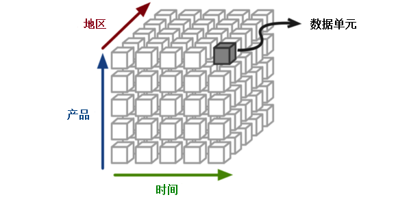
Figure 1
2. Classification
Online analytical processing systems can generally be classified into MOLAP, ROLAP, and HOLAP.(1)MOLAP
MOLAP (multi-dimensional online analytical processing) is a typical form of OLAP and is sometimes even used to represent OLAP.MOLAP stores data in an optimized multidimensional array rather than in a relational database.Some MOLAP tools require precomputing and storing the calculated result data, which is called preprocessing.The MOLAP tool generally collaborates the predicted datasets into a single data cube.For a given range of questions, the data in the cube contains all possible answers.The advantage of preprocessing is that you can respond very quickly to problems.On the other hand, depending on the anticipated aggregation level, loading new data can take a long time.Other MOLAP tools, especially those that implement certain database functions, do not precompute the original data but do so only when needed.
The advantages of MOLAP:
- Fast query performance with optimized data storage, multidimensional data indexing, and caching.
- Compression technology allows data storage to require less disk space than relational databases.
- MOLAP tools generally automate high-level data aggregation.
- Data collections with low cardinality dimensions are compact.
- Array models provide native indexing capabilities.
- Processing steps in some MOLAP solutions can take a long time, especially when there is a large amount of data.To solve this problem, you can usually only incrementally process the changing data, not preprocess the entire data collection.
- More data redundancy may be introduced.
Business OLAP products include Cognos Powerplay, Oracle Database OLAP Option, MicroStrategy, Microsoft Analysis Services, Essbase, etc.
(2)ROLAP
ROLAP stores data directly using a relational database and does not require precomputing.The underlying fact data and its dimension tables are stored as relational tables, while aggregated information is stored in newly created additional tables.ROLAP is based on database schema design and operates on data stored in relational databases to implement traditional OLAP data slicing and blocking functions.Essentially, each data slicing or blocking behavior is the same as adding a filter condition to a "WHERE" clause in an SQL statement.ROLAP does not use a pre-computed data cube, but instead queries standard relational database tables to return the data needed to answer questions.Unlike the predicted MOLAP, the ROLAP tool has the ability to answer any relevant data analysis question because the technology is not limited by cube content.ROLAP also allows you to drill down to the most detailed data stored in the database.
Because ROLAP uses relational databases, database schemas must generally be carefully designed.The databases designed for OLTP applications cannot be used directly as ROLAP databases, and this speculative trick does not make ROLAP work well.Therefore, ROLAP still needs to create additional data copies.However, ROLAP uses a database after all, and a variety of database design and optimization techniques can be effectively used.
Strengths of ROLAP:
- ROLAP is more scalable when dealing with large amounts of data, especially when the dimensions contained in the model have very high cardinalities, such as millions of members in the dimension table.
- There are many data loading tools available, and ETL code can be fine-tuned for a specific data model, which typically takes less time to load than automated OLAP loading.
- Because the data is stored in a standard relational database, you can use SQL reporting tools to access the data instead of a proprietary OLAP tool.
- ROLAP is better suited for dealing with non-aggregated facts, such as text descriptions.Performance is relatively poor when querying text-type elements in MOLP tools.
- By decoupling data storage from a multidimensional model, this more general relationship model increases the likelihood of successful modeling than using a rigorous dimension model.
- The ROLAP method can take advantage of database privilege control, such as row-level security settings, to filter query results using pre-set conditions.For example, Oracle's VPD technology can automatically stitch WHERE predicate conditions in query SQL statements based on connected users.
- It is generally accepted that ROLAP tools are slower than MOLAP queries.
- Data loading of aggregation tables must be controlled by user-customized ETL code.ROLAP tools cannot automate this task, which means additional development work.
- If you skip the step of creating aggregate tables, query performance will be compromised because you will have to query a large number of detail tables.Although performance problems can be alleviated by properly establishing aggregation tables, it is impractical to create aggregation tables for a combination of all dimension tables and their attributes.
- ROLAP relies on databases that target common queries or caches, and therefore does not provide the special techniques that some MOLAP tools have, such as pivot tables.However, modern ROLAP tools can take advantage of CUBE, ROLLUP operations or other SQL OLAP extensions in the SQL language.With the gradual improvement of these SQL extensions, the advantages of MOLAP tools are less obvious.
- Because all the calculations of the ROLAP tool depend on SQL, ROLAP is no longer applicable for some computation-intensive models that are not easily converted to SQL.Examples include complex financial statements with items such as budgets, appropriations, or scenarios for geographic location calculations.
Business products using ROLAP include Microsoft Analysis Services, MicroStrategy, SAP Business Objects, Oracle Business Intelligence Suite Enterprise Edition, Tableau Software, etc.There are also open source ROLAP servers, such as Mondrian.
(3)HOLAP
* It is difficult to choose between additional ETL development costs and slow query performance because most commercial OLAP tools now use a Hybrid method that allows model designers to decide which data is stored in MOLAP and which in ROLAP.In addition to dividing data into traditional relational and proprietary storage, the industry does not have a clear definition of hybrid OLAP.For example, some vendors'OLAP databases use relational tables to store a large amount of detailed data, but specialized tables to store a small amount of aggregated data.HOLAP combines the advantages of both MOLAP and ROLAP methods to utilize both the predicted multidimensional cube and the relational data source.HOLAP has two strategies for dividing data.
- Vertical partition.HOLAP in this mode stores aggregated data in MOLAP to support good query performance while storing detailed data in ROLAP to reduce the time required for cube processing.
- Horizontal partition.This mode of HOLAP divides by data warmth, storing some recently used data fragments in MOLAP and older data in ROLAP.
3. Performance
The amount of raw data required for OLAP analysis is enormous.An analysis model often involves tens of millions or hundreds of millions or more data, and the analysis model contains multiple dimension data, which can be arbitrarily combined by users.The result is that a large number of real-time operations result in excessive response times.Imagine an analysis model of 10 million records. If you extract four dimensions at a time for combinatorial analysis, each dimension has 10 different values, and the theoretical number of operations will reach 12 times of 10.This amount of computation can result in tens of minutes or longer wait times.If the user adjusts the order of dimension combinations, or increases or decreases some dimensions, it will be a recalculation process.From the above analysis, it can be concluded that OLAP will only be a concept of no practical value if the operational efficiency of OLAP cannot be solved.In the history of OLAP, a common solution is to use multidimensional database instead of relational database design, to aggregate data to the maximum extent according to the dimensions, taking into account various combinations of dimensions. The result of the operation will be a data cube, which will be saved on disk, and this pre-operation will speed up OLAP.For example, Kylin uses this space-for-time method to improve query speed, and the performance advantages of HAWQ make it more suitable for OLAP applications.For performance comparison between HAWQ and Hive, see "HAWQ versus Hive Query Performance Test".(http://blog.csdn.net/wzy0623/article/details/71479539)
2. OLAP Instances
A thorough understanding of business data is required to make good use of OLAP classes.Understanding the business is the key to knowing which metrics need to be analyzed so that relevant data can be analyzed in a targeted manner and credible conclusions can be drawn to assist in decision making.Following is an example of a sales order data warehouse, where several questions are raised, and HAWQ is used to query the data to answer these questions:- What is the cumulative sales and sales of each product type and individual products?
- What are the monthly sales and sales trends for each product type and individual product in each province and city?
- What are the sales and sales volumes and the same for each product type?
- What is the total number of customers and their remittance for consumption in each province and city?
- What is the percentage of late orders?
- What is the average and median annual customer spending?
- What is the annual consumption amount of customers at 25%, 50%, 75% locations?
- What is the proportion of the number of customers with high, medium and low annual consumption amounts and consumption amounts?
- What are the top three items by sales amount in each city?
- Percentage ranking of sales for all products?
1. What is the cumulative sales and sales of each product type and individual products?
Subtotal and total using group by rollup of HAWQ.dw=> select t2.product_category, t2.product_name, sum(nq), sum(order_amount)
dw-> from v_sales_order_fact t1, product_dim t2
dw-> where t1.product_sk = t2.product_sk
dw-> group by rollup (t2.product_category, t2.product_name)
dw-> order by t2.product_category, t2.product_name;
product_category | product_name | sum | sum
------------------+-----------------+-----+-----------
monitor | flat panel | | 49666.00
monitor | lcd panel | 11 | 3087.00
monitor | | 11 | 52753.00
peripheral | keyboard | 38 | 67387.00
peripheral | | 38 | 67387.00
storage | floppy drive | 52 | 348655.00
storage | hard disk drive | 80 | 375481.00
storage | | 132 | 724136.00
| | 181 | 844276.00
(9 rows)2. What is the monthly sales and sales of each product type and individual product in each province and city?
The query statement is similar to the previous question except that it has more zip dimension tables associated with it and adds two columns, province and city, to the group by rollup.dw=> select t2.product_category, t2.product_name, t3.state, t3.city, sum(nq), sum(order_amount)
dw-> from v_sales_order_fact t1, product_dim t2, zip_code_dim t3
dw-> where t1.product_sk = t2.product_sk
dw-> and t1.customer_zip_code_sk = t3.zip_code_sk
dw-> group by rollup (t2.product_category, t2.product_name, t3.state, t3.city)
dw-> order by t2.product_category, t2.product_name, t3.state, t3.city;
product_category | product_name | state | city | sum | sum
------------------+-----------------+-------+---------------+-----+-----------
monitor | flat panel | oh | cleveland | | 7431.00
monitor | flat panel | oh | | | 7431.00
monitor | flat panel | pa | mechanicsburg | | 10630.00
monitor | flat panel | pa | pittsburgh | | 31605.00
monitor | flat panel | pa | | | 42235.00
monitor | flat panel | | | | 49666.00
monitor | lcd panel | pa | pittsburgh | 11 | 3087.00
monitor | lcd panel | pa | | 11 | 3087.00
monitor | lcd panel | | | 11 | 3087.00
monitor | | | | 11 | 52753.00
peripheral | keyboard | oh | cleveland | 38 | 10875.00
peripheral | keyboard | oh | | 38 | 10875.00
peripheral | keyboard | pa | mechanicsburg | | 29629.00
peripheral | keyboard | pa | pittsburgh | | 26883.00
peripheral | keyboard | pa | | | 56512.00
peripheral | keyboard | | | 38 | 67387.00
peripheral | | | | 38 | 67387.00
storage | floppy drive | oh | cleveland | | 8229.00
storage | floppy drive | oh | | | 8229.00
storage | floppy drive | pa | mechanicsburg | | 140410.00
storage | floppy drive | pa | pittsburgh | 52 | 200016.00
storage | floppy drive | pa | | 52 | 340426.00
storage | floppy drive | | | 52 | 348655.00
storage | hard disk drive | oh | cleveland | | 8646.00
storage | hard disk drive | oh | | | 8646.00
storage | hard disk drive | pa | mechanicsburg | 80 | 194444.00
storage | hard disk drive | pa | pittsburgh | | 172391.00
storage | hard disk drive | pa | | 80 | 366835.00
storage | hard disk drive | | | 80 | 375481.00
storage | | | | 132 | 724136.00
| | | | 181 | 844276.00
(31 rows)3. What are the sales and sales volumes and the same for each product type?
The query cycle snapshot v_month_end_sales_order_fact is required.dw=> select t2.product_category, dw-> t1.year_month, dw-> sum(quantity1) quantity_cur, dw-> sum(quantity2) quantity_pre, dw-> round((sum(quantity1) - sum(quantity2)) / sum(quantity2),2) pct_quantity, dw-> sum(amount1) amount_cur, dw-> sum(amount2) amount_pre, dw-> round((sum(amount1) - sum(amount2)) / sum(amount2),2) pct_amount dw-> from (select t1.product_sk, dw(> t1.year_month, dw(> t1.month_order_quantity quantity1, dw(> t2.month_order_quantity quantity2, dw(> t1.month_order_amount amount1, dw(> t2.month_order_amount amount2 dw(> from v_month_end_sales_order_fact t1 dw(> join v_month_end_sales_order_fact t2 dw(> on t1.product_sk = t2.product_sk dw(> and t1.year_month/100 = t2.year_month/100 + 1 dw(> and t1.year_month - t1.year_month/100*100 = t2.year_month - t2.year_month/100*100) t1, dw-> product_dim t2 dw-> where t1.product_sk = t2.product_sk dw-> group by t2.product_category, t1.year_month dw-> order by t2.product_category, t1.year_month; product_category | year_month | quantity_cur | quantity_pre | pct_quantity | amount_cur | amount_pre | pct_amount ------------------+------------+--------------+--------------+--------------+------------+------------+------------ storage | 201705 | 943 | | | 142814.00 | 110172.00 | 0.30 storage | 201706 | 110 | | | 9132.00 | 116418.00 | -0.92 (2 rows)
4. How many customers and their consumption remittances are there in each province and city?
dw=> select t2.state,
dw->        t2.city,
dw->        count(distinct customer_sk) sum_customer_num,
dw->        sum(order_amount) sum_order_amount
dw->   from v_sales_order_fact t1, zip_code_dim t2
dw->  where t1.customer_zip_code_sk = t2.zip_code_sk
dw->  group by rollup (t2.state, t2.city)
dw->  order by t2.state, t2.city;
 state |     city      | sum_customer_num | sum_order_amount
-------+---------------+------------------+------------------
 oh    | cleveland     |                4 |         35181.00
 oh    |               |                4 |         35181.00
 pa    | mechanicsburg |                8 |        375113.00
 pa    | pittsburgh    |               12 |        433982.00
 pa    |               |               20 |        809095.00
       |               |               24 |        844276.00
(6 rows)
5. What is the percentage of late orders?
Note that sum_late needs to be explicitly converted to a numeric data type.dw=> select sum_total, sum_late, round(cast(sum_late as numeric)/sum_total,4) late_pct
dw-> from (select sum(case when status_date_sk < entry_date_sk then 1
dw(> else 0
dw(> end) sum_late,
dw(> count(*) sum_total
dw(> from sales_order_fact) t;
sum_total | sum_late | late_pct
-----------+----------+----------
151 | 2 | 0.0132
(1 row)6. What is the average and median annual customer spending?
Averages and medians are calculated using two methods.HAWQ provides a rich set of aggregation functions for analytical applications.dw=> select round(avg(sum_order_amount),2) avg_amount, dw-> round(sum(sum_order_amount)/count(customer_sk),2) avg_amount1, dw-> percentile_cont(0.5) within group (order by sum_order_amount) median_amount, dw-> median(sum_order_amount) median_amount1 dw-> from (select customer_sk,sum(order_amount) sum_order_amount dw(> from v_sales_order_fact dw(> group by customer_sk) t1; avg_amount | avg_amount1 | median_amount | median_amount1 ------------+-------------+---------------+---------------- 35178.17 | 35178.17 | 14277 | 14277 (1 row)
7. What is the annual consumption amount of customers at 25%, 50%, 75% locations?
dw=> select percentile_cont(0.25) within group (order by sum_order_amount desc) max_amount_25,
dw->        percentile_cont(0.50) within group (order by sum_order_amount desc) max_amount_50,
dw->        percentile_cont(0.75) within group (order by sum_order_amount desc) max_amount_75
dw->   from (select customer_sk,sum(order_amount) sum_order_amount
dw(>           from v_sales_order_fact
dw(>          group by customer_sk) t1;
 max_amount_25 | max_amount_50 | max_amount_75
---------------+---------------+---------------
       50536.5 |         14277 |       8342.25
(1 row)
8. What is the proportion of the number of customers with high, medium and low annual consumption amounts and consumption amounts?
Use in HAWQ Replaces Traditional Number Warehouse Practice (12) - Dimension Dimension by Dimension Table Technology "To query by segments defined in.dw=> select year1, dw-> bn, dw-> c_count, dw-> sum_band, dw-> sum_total, dw-> round(sum_band/sum_total,4) band_pct dw-> from (select count(a.customer_sk) c_count, dw(> sum(annual_order_amount) sum_band, dw(> a.year year1, dw(> band_name bn dw(> from annual_customer_segment_fact a, dw(> annual_order_segment_dim b, dw(> annual_sales_order_fact d dw(> where a.segment_sk = b.segment_sk dw(> and a.customer_sk = d.customer_sk dw(> and a.year = d.year dw(> and b.segment_name = 'grid' dw(> group by a.year, bn) t1, dw-> (select sum(annual_order_amount) sum_total dw(> from annual_sales_order_fact) t2 dw-> order by year1, bn; year1 | bn | c_count | sum_band | sum_total | band_pct -------+------+---------+-----------+-----------+---------- 2016 | high | 6 | 572190.00 | 572190.00 | 1.0000 (1 row)
9. What are the top three goods by sales amount in each city?
Use the window function row_number() provided by HAWQ to rank sales in reverse order by city division.dw=> select case when t1.rn =1 then t1.city end city,
dw-> t2.product_name,
dw-> t1.sum_order_amount,
dw-> t1.rn
dw-> from (select city,
dw(> product_sk,
dw(> sum_order_amount,
dw(> row_number() over (partition by city order by sum_order_amount desc) rn
dw(> from (select t2.state||':'||t2.city city,
dw(> product_sk,
dw(> sum(order_amount) sum_order_amount
dw(> from v_sales_order_fact t1, zip_code_dim t2
dw(> where t1.customer_zip_code_sk = t2.zip_code_sk
dw(> group by t2.state||':'||t2.city, product_sk) t) t1
dw-> inner join product_dim t2 on t1.product_sk = t2.product_sk
dw-> where t1.rn <= 3
dw-> order by t1.city, t1.rn;
city | product_name | sum_order_amount | rn
------------------+-----------------+------------------+----
oh:cleveland | keyboard | 10875.00 | 1
| hard disk drive | 8646.00 | 2
| floppy drive | 8229.00 | 3
pa:mechanicsburg | hard disk drive | 194444.00 | 1
| floppy drive | 140410.00 | 2
| keyboard | 29629.00 | 3
pa:pittsburgh | floppy drive | 200016.00 | 1
| hard disk drive | 172391.00 | 2
| flat panel | 31605.00 | 3
(9 rows)10. Percentage ranking of sales of all products?
dw=> select product_name,
dw->        sum_order_amount,
dw->        percent_rank() over (order by sum_order_amount desc) rank
dw->   from (select product_sk,sum(order_amount) sum_order_amount
dw(>           from v_sales_order_fact
dw(>          group by product_sk) t1, product_dim t2
dw->  where t1.product_sk = t2.product_sk
dw->  order by rank;
  product_name   | sum_order_amount | rank
-----------------+------------------+------
 hard disk drive |        375481.00 |    0
 floppy drive    |        348655.00 | 0.25
 keyboard        |         67387.00 |  0.5
 flat panel      |         49666.00 | 0.75
 lcd panel       |          3087.00 |    1
(5 rows)
3. Interactive Query and Graphical Display
1. Introduction to Zeppelin
Zeppelin is a Web-based software for interactive data analysis.It started as an incubator project for the Apache Software Foundation and became a top-level project in May 2016.Zeppelin describes himself as a notebook that allows data ingestion, data discovery, data analysis, and data visualization to help developers, data scientists, and related users process data more effectively without having to use complex command lines or care about the implementation details of clusters.The architecture of Zeppelin is shown in Figure 2.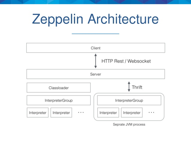
Figure 2
As you can see from the above image, Zeppelin has a client/server architecture, and the client is generally a browser.The server receives the client's request and sends it to the translator group through the Thrift protocol.The translator group is physically represented as a JVM process and is responsible for actually handling client requests and communicating with the server.
Translator is a plug-in architecture that allows any language or back-end data processor to be added to Zeppelin as a plug-in.In particular, Zeppelin has a built-in Spark translator, so there is no need to build separate modules, plug-ins, or libraries.The architecture of the translator is shown in Figure 3.
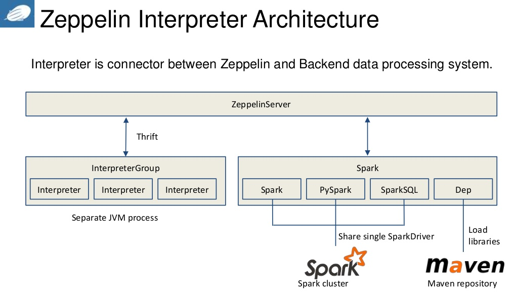
Figure 3
Current Zeppelin supports many translators, such as alluxio, cassandra, file, hbase, ignite, kylin, md, phoenix, sh, tajo, angular, elastic search, flink, hive, jdbc, lens, psql, spark and so on.Plug-in architecture allows users to use specific programming languages or data processing methods that they are familiar with in Zeppelin.For example, you can use Scala language code in Zeppelin by using the%spark translator.
In data visualization, Zeppelin already contains some basic graphs, such as histograms, pie charts, line charts, scatterplots, etc. Any supported back-end language output can be represented graphically.
In Zeppelin, each query created by a user is called a note, and the URL of note is shared among multiple users, and Zeppelin broadcasts changes to note to all users in real time.Zeppelin also provides a URL that shows only the results of the query, which does not include any menus and buttons.In this way, you can easily embed the result page as a frame in your own web site.
2. Execute HAWQ queries using Zeppelin
(1) Install Zeppelin* Zeppelin 0.6.0 has been integrated into the HDP 2.5.0 installation package, so complex installation configurations are not required separately, as long as the Zeppelin service is started.
(2) Configure Zeppelin support for HAWQ
Zeppelin 0.6.0 parses HAWQ queries through a JDBC translator with simple configuration steps as follows.
- On the Ambari console home page, click Services -> Zeppelin Notebook -> Quick Links -> Zeppelin UI to open the Zeppelin UI home page.
- On the Zeppelin UI home page, click anonymous -> interpreter to enter the translator page.
- Click edit to edit the jdbc translator and configure the values of default.driver, default.password, default.url, default.user, as shown in Figure 4.
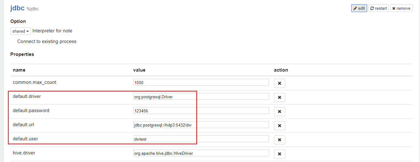
Figure 4
- Once configured, click Save to save the configuration, and then click restart to restart the jdbc translator until the configuration is complete.
Click Notebook -> Create new note to create a new note, where you enter query statements such as "What is the monthly sales and sales of each product type and individual product in each province and city?"Queries for.
Tables, columns, pies, stacks, lines, and scatterplots of the results of the run are shown in Figures 5-10, respectively.%jdbc select t2.product_category, t2.product_name, t3.state, t3.city, sum(nq) sq, sum(order_amount) sa from v_sales_order_fact t1, product_dim t2, zip_code_dim t3 where t1.product_sk = t2.product_sk and t1.customer_zip_code_sk = t3.zip_code_sk group by t2.product_category, t2.product_name, t3.state, t3.city order by t2.product_category, t2.product_name, t3.state, t3.city;
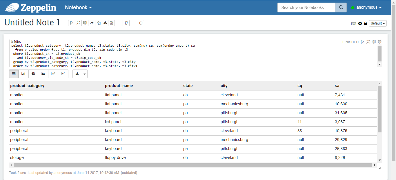
Figure 5
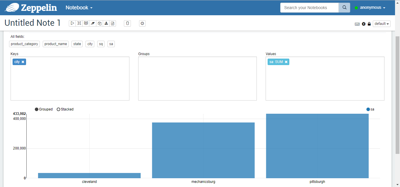
Figure 6
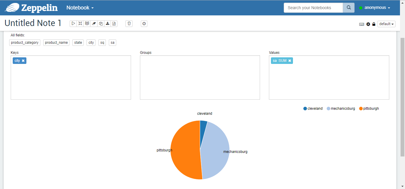
Figure 7
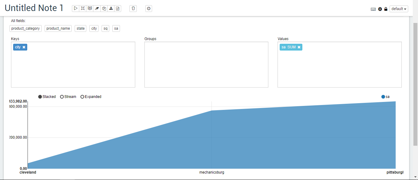
Figure 8
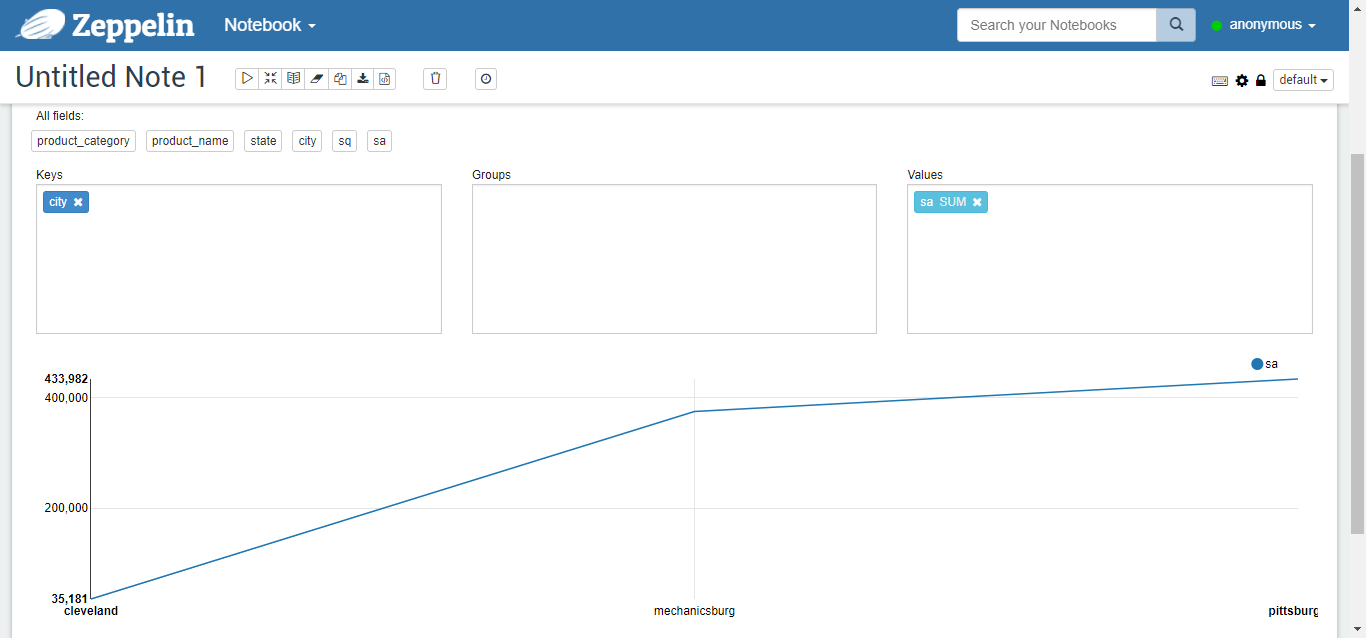
Figure 9
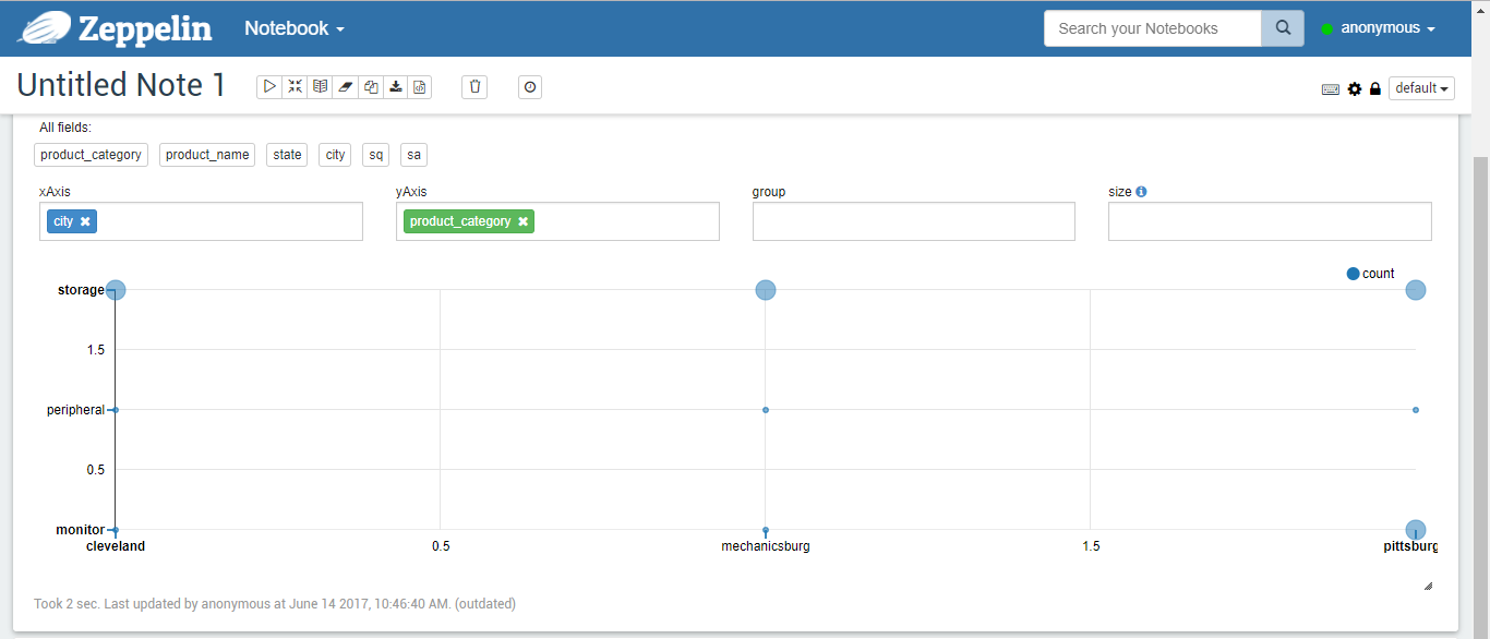
Figure 10
Multiple query statements can be executed independently in a note.The graphical display can analyze different metrics online based on different "settings".There are three optional styles for reports: default, simple, and report.For example, a pie chart representation of a report style is shown in Figure 11.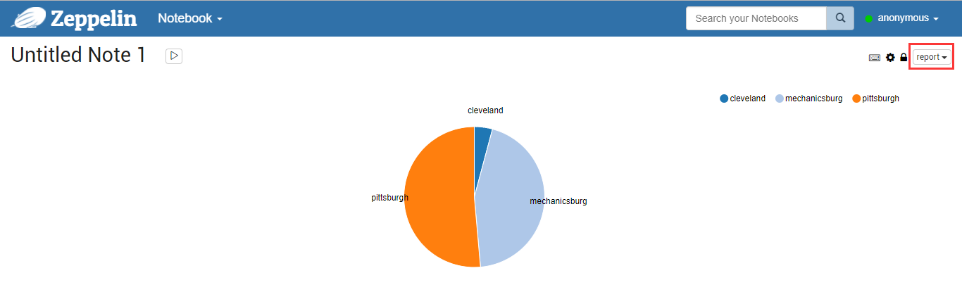
Figure 11
You can reference this report separately by clicking on the link shown in the red box in Figure 12.
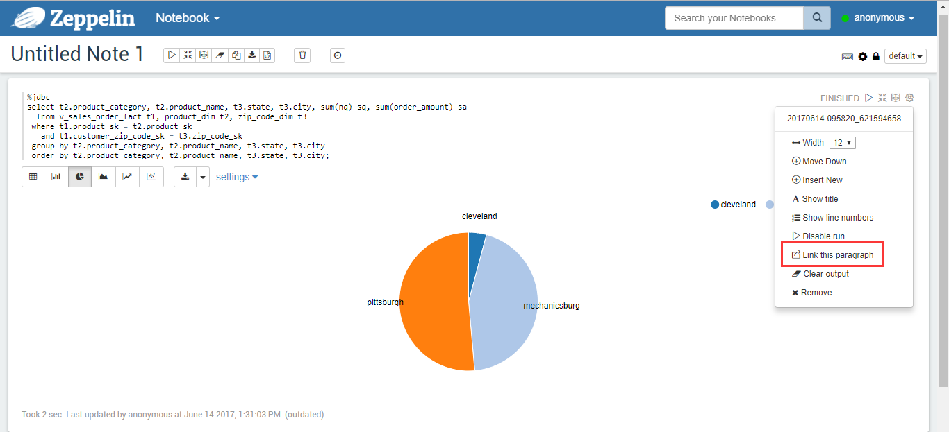
Figure 12
Separate pages can change in real time depending on changes to queries or settings, such as changing Values from sa to sq columns and pie charts to look like Figure 13.
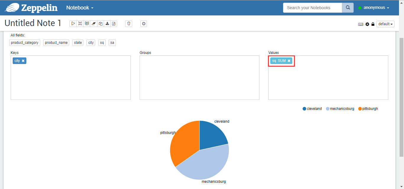
Figure 13
Separate linked pages also change automatically, as shown in Figure 14.
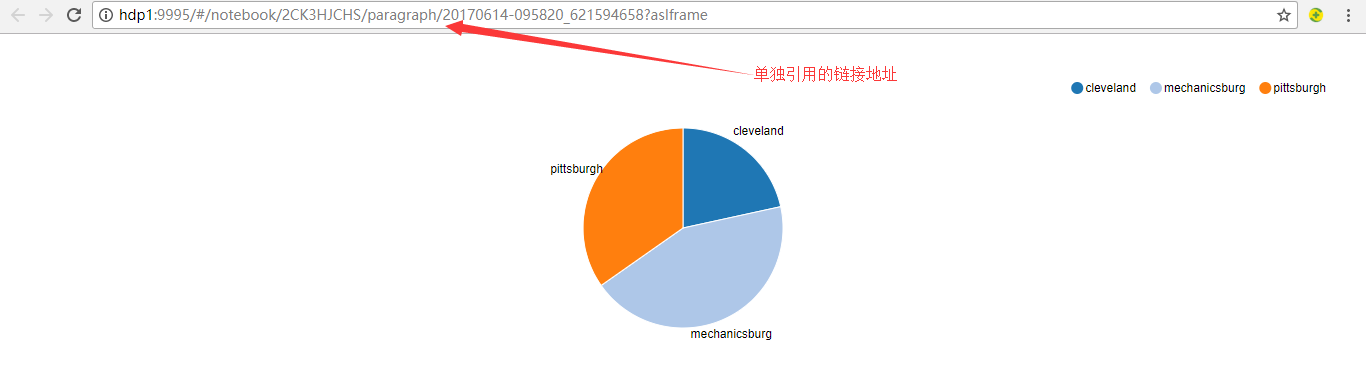
Figure 14
Zeppelin supports online input of variable values, for example, to query sales for a certain year, change the query statement to:
%jdbc
select t2.product_category, t2.product_name, t3.state, t3.city, sum(nq) sq, sum(order_amount) sa
  from v_sales_order_fact t1, product_dim t2, zip_code_dim t3
 where t1.product_sk = t2.product_sk
   and t1.customer_zip_code_sk = t3.zip_code_sk
   and t1.year_month/100 = ${year}
 group by t2.product_category, t2.product_name, t3.state, t3.city
 order by t2.product_category, t2.product_name, t3.state, t3.city;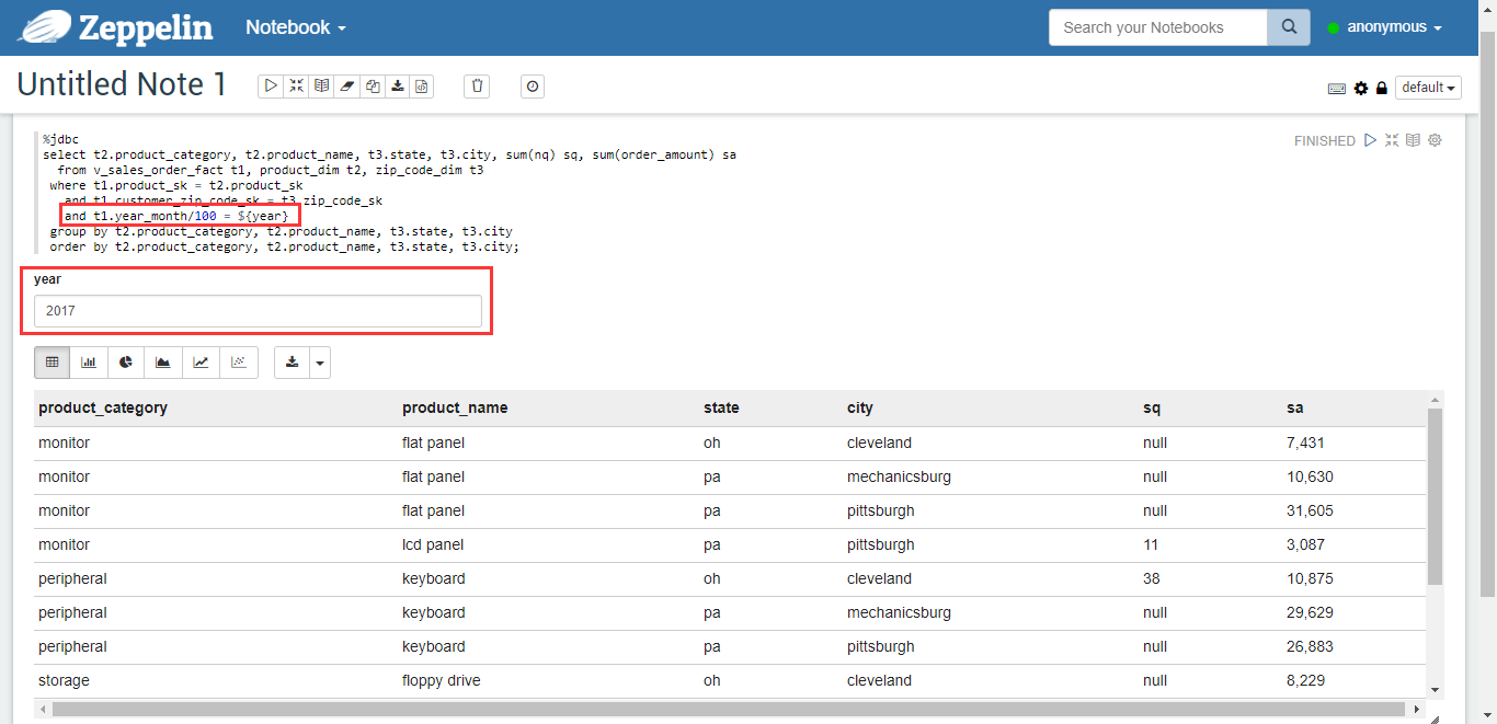
Figure 15
You can even dynamically define the columns of a query, such as changing the query statement to:
%jdbc
select ${checkbox:fields=t2.product_category, t2.product_category|t2.product_name},t3.state, t3.city, sum(nq) sq, sum(order_amount) sa
  from v_sales_order_fact t1, product_dim t2, zip_code_dim t3
 where t1.product_sk = t2.product_sk
   and t1.customer_zip_code_sk = t3.zip_code_sk
   and t1.year_month/100 = ${year}
 group by ${checkbox:fields=t2.product_category, t2.product_category|t2.product_name}, t3.state, t3.city
 order by ${checkbox:fields=t2.product_category, t2.product_category|t2.product_name}, t3.state, t3.city;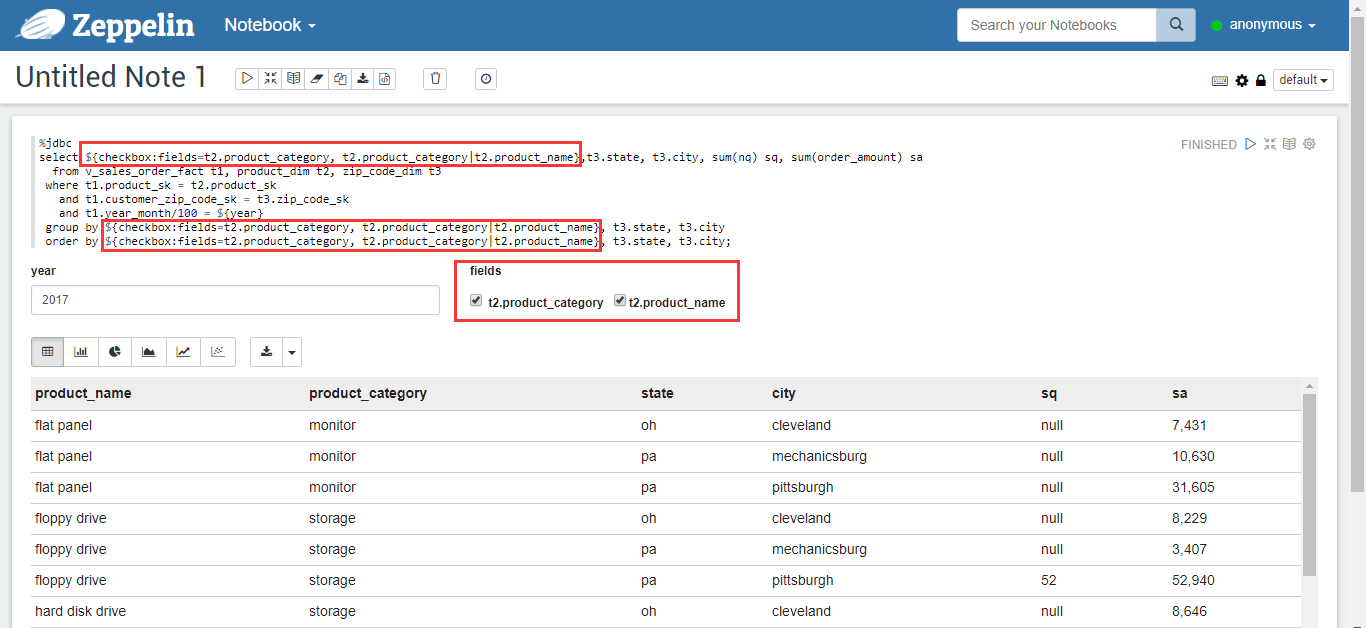
Figure 16
Reference: https://zeppelin.apache.org/docs/latest/manual/dynamicform.html