introduce

No matter how powerful, machine learning cannot predict everything. For example, in the field related to time series prediction, the performance is not very good.
Although a large number of autoregressive models and many other time series algorithms are available, the target distribution cannot be predicted if the target distribution is white noise or follows random walk.
Therefore, you must detect such distributions before making further efforts.
In this article, you will learn what white noise and random walk are and explore proven statistical techniques to detect them.
Brief description of autocorrelation
Autocorrelation involves finding the correlation between a time series and its own lagged version. Consider this distribution:
deg_C = tps_july["deg_C"].to_frame("temperature")
deg_C.head()

Lag time series means moving it back one or more cycles:
deg_C["lag_1"] = deg_C["temperature"].shift(periods=1)
deg_C["lag_2"] = deg_C["temperature"].shift(periods=2)
deg_C["lag_3"] = deg_C["temperature"].shift(periods=3)

deg_C.head(6)
The autocorrelation function (ACF) finds the correlation coefficient between the time series and its lagged version at each lag k. You can use plot in stats models_ The ACF function draws it. This is what it looks like:
from matplotlib import rcParams
from statsmodels.graphics.tsaplots import plot_acf

rcParams["figure.figsize"] = 9, 4
# ACF function up to 50 lags
fig = plot_acf(deg_C["temperature"], lags=50)

plt.show();
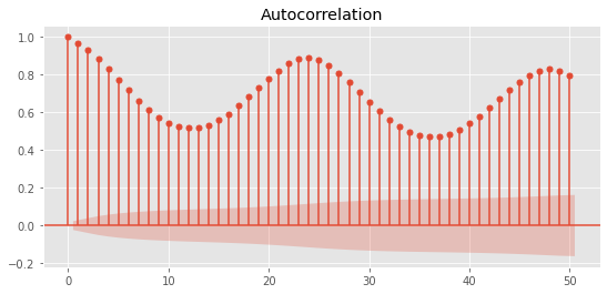
XAxis is the lag k and YAxis is the Pearson correlation coefficient for each lag. The red shaded area is the confidence interval. If the height of the bar is outside the region, it means that the correlation is statistically significant.
What is white noise?
In short, the white noise distribution is any distribution with the following characteristics:
- Zero mean
- Constant variance / standard deviation (not changing over time)
- Zero autocorrelation of all lags
In essence, it is a series of random numbers. By definition, no algorithm can reasonably model its behavior.
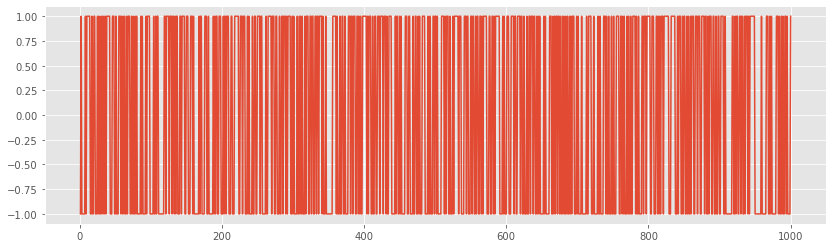
There are special types of white noise. If the noise is normal (subject to normal distribution), it is called Gaussian white noise. Let's take a visual look at an example:
noise = np.random.normal(loc=0, scale=0.5, size=1000)

plt.figure(figsize=(12, 4))
plt.plot(noise);
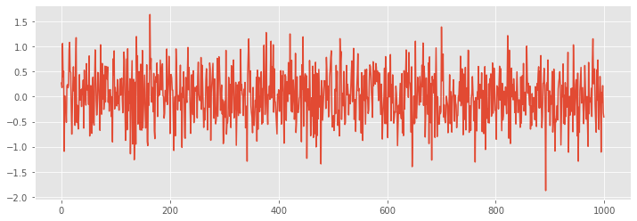
Even if there are occasional spikes, there is no obvious pattern, that is, the distribution is completely random.
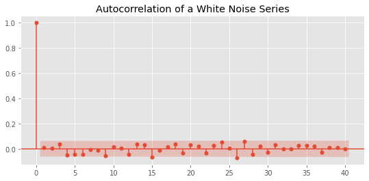
The best way to verify this is to create an ACF diagram:
fig = plot_acf(noise, lags=40)

plt.title("Autocorrelation of a White Noise Series")
plt.show()
There are also "strict" white noise distributions - their sequence correlation is strictly 0. This is different from Brown / pink noise or other natural random phenomena, in which there is weak sequence correlation but still no memory.
The importance of white noise in prediction and model diagnosis

Although white noise distributions are considered dead ends, they are also very useful in other cases.
For example, in time series prediction, if the difference between the predicted value and the actual value represents the white noise distribution, you can be glad that you have done a good job.
When the residual shows any pattern, whether seasonal, trend or non-zero mean, it indicates that there is still room for improvement. In contrast, if the residual is pure white noise, you maximize the capability of the selected model.
In other words, the algorithm tries to capture all important signals and attributes of the target. The rest are random fluctuations and inconsistent data points that cannot be attributed to anything.
For example, we will use the July Kaggle playground competition to predict the content of carbon monoxide in the air. We will keep the input "as is" - we will not perform any feature engineering, we will select a baseline model with default parameters:
preds = forest.predict(X_test)
residuals = y_test.flatten() - preds

plt.plot(residuals)
plt.title("Plot of the Error residuals");
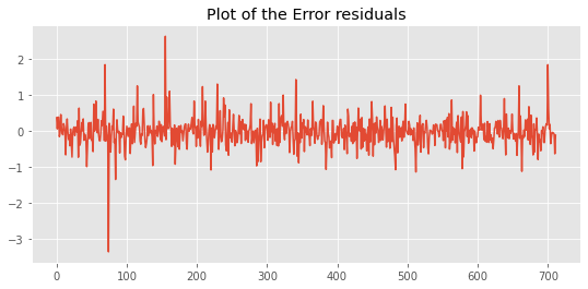
fig = plot_acf(residuals, lags=50)

plt.title("Autocorrelation Plot of the Error residuals")
plt.show();
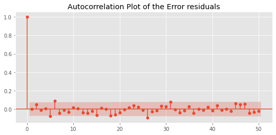
There are some patterns in the ACF diagram, but they are within the confidence interval. These two figures show that even with the default parameters, the random forest can capture almost all important signals from the training data.
Random walk
The more challenging but equally unpredictable distribution in time series prediction is random walk. Unlike white noise, it has non-zero mean, non constant standard / variance, and looks like a regular distribution when plotted:
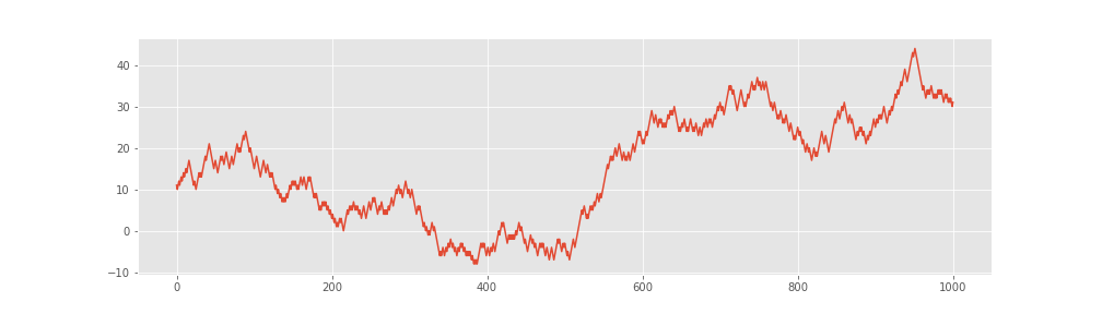
Random walk series are always cleverly disguised in this way, but they are still unpredictable. The best guess for today's value is yesterday's value.
A common puzzle for beginners is to regard random walk as a simple sequence of random numbers. This is not the case, because in random walk, each step depends on the previous step.
Therefore, the autocorrelation function of random walk does return non-zero correlation.
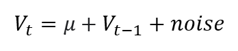
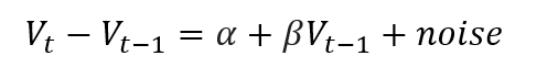
The formula for random walk is simple:
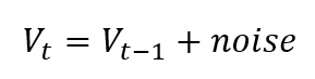
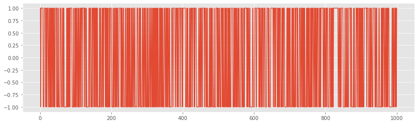
No matter what the previous data point is, you can add some random values to it and continue as needed. Let's generate it in Python. The starting value is 99:
walk = [99]

for i in range(1000):
    # Create random noise
    noise = -1 if np.random.random() < 0.5 else 1
    walk.append(walk[-1] + noise)

rcParams["figure.figsize"] = 14, 4
plt.plot(walk);
Let's also draw ACF:
fig = plot_acf(walk, lags=50)
plt.show();
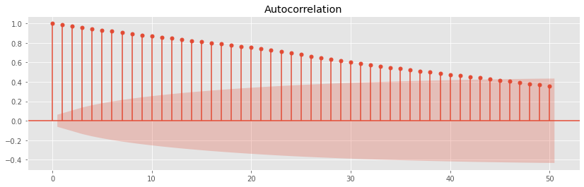
As you can see, the first 40 lags produce statistically significant correlations.
So how do we detect random walk when visualization is not an option?
Due to the way they are created, the difference of time series should isolate the random addition of each step. The first-order difference is obtained by delaying the sequence by 1 and subtracting it from the original value. Pandas has a convenient diff function to do this:
walk_diff = pd.Series(walk).diff()

plt.plot(walk_diff);
If the first-order difference of the time series is plotted and the result is white noise, it is a random walk.
Random walk with drift
A slight modification to the conventional random walk is to add a constant value called drift to the random step:
Drift is usually used μ In terms of time-varying values, drift means gradually becoming something.
For example, even if stocks fluctuate continuously, they may also have a positive drift, that is, they gradually increase as a whole over time.
Now let's see how to simulate this in Python. We will first create a regular random walk with a starting value of 25:
walk = [25]

for i in range(1000):
    # Create random noise
    noise = -1 if np.random.random() < 0.5 else 1
    walk.append(walk[-1] + noise)
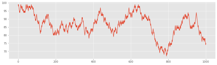
From the above formula, we can see that we need to add the required drift at each step. Let's add a drift of 5 and view the plot:
drift = 5
drifty_walk = pd.Series(walk) + 5

drifty_walk.plot(title="A Random Walk with Drift");
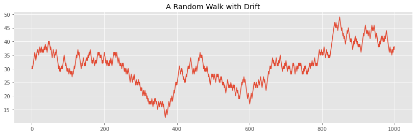
Despite the sharp fluctuations, the series still has an obvious upward trend. If we perform the difference, we will see that the series is still random walk:
drifty_walk.diff().plot();
Statistical detection random walk
You might ask if there is a better way to identify random walks than just "observe" them from the graph.
As an answer, Dicker D. A. and Fuller W. A. outlined a hypothesis test in 1979, which is called the augmented Dickey fuller test.
In essence, it attempts to test a series of null hypotheses that follow random walk. Behind the scenes, it regresses the price difference of the lagging price.
If you find the slope of( β) Equal to 0, the series is random walk. If the slope is significantly different from 0, we reject the original assumption that the series follows random walk.
Fortunately, you don't have to worry about math because the test is already implemented in Python.
We import the adfuller function from statsmodels and use it for the drift random walk created in the previous section:
from statsmodels.tsa.stattools import adfuller

results = adfuller(drifty_walk)

print(f"ADF Statistic: {results[0]}")
print(f"p-value: {results[1]}")
print("Critical Values:")
for key, value in results[4].items():
    print("\t%s: %.3f" % (key, value))

----------------------------------------------

ADF Statistic: -2.0646595557153424
p-value: 0.25896047143602574
Critical Values:
	1%: -3.437
	5%: -2.864
	10%: -2.568
Let's look at the p value, which is about 0.26. Since 0.05 is the significance threshold, we cannot reject the drift_ Walk is the null hypothesis of random walk, that is, it is random walk.
Let's do another test for distributions that we know are not random walks. We will use the carbon monoxide goals of the TPS July Kaggle amusement park competition:
results = adfuller(tps_july["target_carbon_monoxide"])

print(f"ADF Statistic: {results[0]}")
print(f"p-value: {results[1]}")
print("Critical Values:")
for key, value in results[4].items():
    print("\t%s: %.3f" % (key, value))

---------------------------------------------------

ADF Statistic: -8.982102584771997
p-value: 7.26341357249666e-15
Critical Values:
	1%: -3.431
	5%: -2.862
	10%: -2.567
The p value is very small, which indicates that we can easily reject the target_carbon_monoxide follows the original hypothesis of random walk.
Author: Bex T
3f" % (key, value))
ADF Statistic: -8.982102584771997
p-value: 7.26341357249666e-15
Critical Values:
1%: -3.431
5%: -2.862
10%: -2.567
p The value is very small, indicating that we can easily refuse target_carbon_monoxide Follow the original hypothesis of random walk.

Author: Bex T.