In this article, we will see how to deal with the regression problem and how to improve the accuracy of machine learning model by using the concepts of feature transformation, feature engineering, clustering, enhancement algorithm and so on.

Data science is an iterative process. Only through repeated experiments can we get the most suitable model / solution for our needs.

Let's focus on each of the above stages through an example. I have a health insurance dataset (CSV file), which contains customer information such as insurance premium, age, gender, BMI, etc. We must predict insurance costs based on these parameters in the data set. This is a regression problem because our target variable - cost / insurance cost - is numeric.

Let's start with loading datasets and exploring attributes (EDA - exploratory data analysis)

#Load csv into a dataframe
df=pd.read_csv('insurance_data.csv')
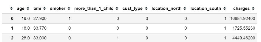
df.head(3)#Get the number of rows and columns
print(f'Dataset size: {df.shape}')
(1338,7)

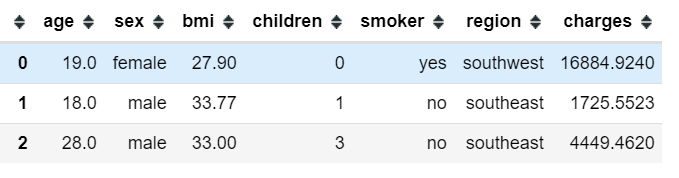
The dataset has 1338 records and 6 characteristics. Smokers, gender and region are categorical variables, while age, BMI and children are numerical variables.

Zero / missing value processing

Let's check the proportion of missing values in the dataset:

df.isnull().sum().sort_values(ascending=False)/df.shape[0]

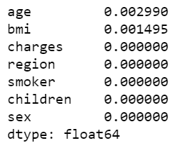
Age and BMI have some zero values - though few. We will process these missing data and then start data analysis. Sklearn's SimpleImputer allows you to replace missing values based on the average / median / most frequent values in their respective columns. In this case, I use the median to fill in the null value.

#Instantiate SimpleImputer 
si=SimpleImputer(missing_values = np.nan, strategy="median")
si.fit(df[['age', 'bmi']])
  
#Filling missing data with median
df[['age', 'bmi']] = si.transform(df[['age', 'bmi']])

Data visualization

Now our data is clean. We will analyze the data through visualization and map. A simple seafood pairing can give us a lot of enlightenment!

sns.pairplot(data=df, diag_kind='kde')

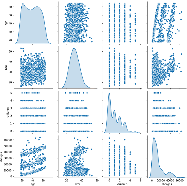
What do we see?

Fees and children are distorted.

Age is positively correlated with fees.

BMI follows normal distribution! 😎

Seaborn's box chart and count chart can be used to reveal the impact of classification variables on charges.

According to the observation of the above figure:

The number of men and women is almost equal, and the average median charge for men and women is the same, but the charge range for men is higher.

Smokers' insurance costs are relatively high.

People with 2-3 children charge the highest

Customers in these four regions are almost evenly distributed, and their fees are almost the same.

The percentage of female smokers is lower than that of male smokers.

Therefore, we can conclude that "smokers" have a considerable impact on insurance costs, while gender has the least impact.

Let's create a heat map to understand the correlation between characteristics (age, BMI and children).

sns.heatmap(df[['age', 'bmi', 'children', 'charges']].corr(), cmap='Blues', annot=True)
plt.show()

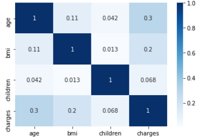
We see an average correlation between age and body mass index and fees.

Now, we will introduce the steps of model preparation and model development one by one.

Feature coding

In this step, we convert the categorical variables - smokers, gender and Region - to digital format (0, 1, 2, 3, etc.), because most algorithms cannot handle non digital data. This process is called coding. There are many ways to do this:

LabelEncoding - represents the classification value as a number (for example, regions with Italian, Indian, US, UK equivalents can be represented as 1, 2, 3, 4)

OrdinalEncoding -- used to represent the ranking based classification data value as a number. (for example, 1,2,3 indicates high, medium and low)

Unique hot coding - represents category data as binary values - only 0 and 1. I prefer to use the unique value in many tags instead of the unique value in the classification. Here, I use a pandas encoding function (get_dummies) on the Region and divide it into four columns - location_NE,location_SE,location_NW and location_SW. Tag coding can also be used in this column, but the single hot coding gives me better results.

#One hot encoding
region=pd.get_dummies(df.region, prefix='location')
df = pd.concat([df,region],axis=1)
df.drop(columns='region', inplace=True)df.sex.replace(to_replace=['male','female'],value=[1,0], inplace=True)
df.smoker.replace(to_replace=['yes', 'no'], value=[1,0], inplace=True)

Feature selection and scaling

Next, we will choose the function that can most affect "charging". I chose all functions except "gender" because it has little impact on the charge (concluded from the chart above). These characteristics will constitute variable X and cost will constitute variable y. If there are many features, I suggest you use scikit learn's SelectKBest for feature selection to reach the top-level features.

#Feature Selection 
y=df.charges.values
X=df[['age', 'bmi', 'smoker', 'children', 'location_northeast', 'location_northwest', 'location_southeast', 'location_southwest']]#Split data into test and train
X_train, X_test, y_train, y_test=train_test_split(X,y, test_size=0.2, random_state=42)

Once we choose our characteristics, we need to "standardize" numbers - age, BMI, children. The standardization process converts the data into smaller values in the range of 0 to 1, so that all values are on the same scale, rather than one overriding the other. I use the StandardScaler here.

#Scaling numeric features using sklearn StandardScalar
numeric=['age', 'bmi', 'children']
sc=StandardScalar()
X_train[numeric]=sc.fit_transform(X_train[numeric])
X_test[numeric]=sc.transform(X_test[numeric])

Now we are ready to create our first basic model 😀. We will try linear regression and decision tree to predict insurance costs

from sklearn.linear_model import LinearRegression
from sklearn.tree import DecisionTreeRegressor
from sklearn.metrics import r2_score, mean_absolute_error, mean_squared_error

#Create a LinearRegression object
lr= LinearRegression()
#Fit X and y 
lr.fit(X_train, y_train)
ypred = lr.predict(X_test)
#Metrics to evaluate your model 
r2_score(y_test, ypred), mean_absolute_error(y_test, ypred), np.sqrt(mean_squared_error(y_test, ypred))


dt = DecisionTreeRegressor()
dt.fit(X_train, y_train)
yhat = dt.predict(X_test)
r2_score(y_test, yhat), mean_absolute_error(y_test, yhat), np.sqrt(mean_squared_error(y_test, yhat))

Mean absolute error (MAE) and root mean square error (RMSE) are the indexes used to evaluate the regression model. You can read more here. Our baseline model gives a score of more than 76%. Between the two methods, decision - trees gives a better Mae of 2780.

Let's see how to make our model better.

Characteristic Engineering

We can improve the model score by manipulating some features in the data set. After several experiments, I found that the following items can improve the accuracy:

Use KMeans to group similar customers into clusters.

In the area column, the northeast and northwest regions are divided into "North" regions, and the southeast and southwest regions are divided into "south" regions.

Convert 'children' to a name called 'more'_ than_ one_ The classification feature of 'child'. If the number of children is > 1, the feature is' Yes'

from sklearn.cluster import KMeans
features=['age', 'bmi', 'smoker', 'children', 'location_northeast', 'location_northwest', 'location_southeast', 'location_southwest']
kmeans = KMeans(n_clusters=2)
kmeans.fit(df[features])

df['cust_type'] = kmeans.predict(df[features])

df['location_north']=df.apply(lambda x: get_north(x['location_northeast'], x['location_northwest']), axis=1

df['location_south']=df.apply(lambda x: get_south(x['location_southwest'], x['location_southeast']), axis=1)

df['more_than_1_child']=df.children.apply(lambda x:1 if x>1 else 0)

Feature transformation

From our EDA, we know that the distribution of "cost" (Y) is highly skewed, so we will apply scikit learn's target transformation - QuantileTransformer to standardize this behavior.

X=df[['age', 'bmi', 'smoker', 'more_than_1_child', 'cust_type', 'location_north', 'location_south']]

#Split test and train data
X_train, X_test, y_train, y_test=train_test_split(X,y, test_size=0.2, random_state=42)

model = DecisionTreeRegressor()
regr_trans = TransformedTargetRegressor(regressor=model, transformer=QuantileTransformer(output_distribution='normal'))
regr_trans.fit(X_train, y_train)
yhat = regr_trans.predict(X_test)
round(r2_score(y_test, yhat), 3), round(mean_absolute_error(y_test, yhat), 2), round(np.sqrt(mean_squared_error(y_test, yhat)),2)

>>0.843, 2189.28, 4931.96

Wow, amazing 84%, MAE has dropped to 2189!

Using integrated and enhanced algorithms

Now we will use the integration of these functions based on random forest, gradient enhancement, LightGBM, and XGBoost. If you are a beginner, you don't realize the methods of boosting and bagging.

X=df[['age', 'bmi', 'smoker', 'more_than_1_child', 'cust_type', 'location_north', 'location_south']]

model = RandomForestRegressor()
#transforming target variable through quantile transformer
ttr = TransformedTargetRegressor(regressor=model, transformer=QuantileTransformer(output_distribution='normal'))
ttr.fit(X_train, y_train)
yhat = ttr.predict(X_test)

r2_score(y_test, yhat), mean_absolute_error(y_test, yhat), np.sqrt(mean_squared_error(y_test, yhat))

>>0.8802, 2078, 4312

yes! Our random forest model performs well - MAE of 2078 👍. Now, we will try some enhancement algorithms, such as gradient enhancement, LightGBM, and XGBoost.

from sklearn.ensemble import GradientBoostingRegressor
import lightgbm
import xgboost

#generic function to fit model and return metrics for every algorithm
def boost_models(x):
    #transforming target variable through quantile transformer
    regr_trans = TransformedTargetRegressor(regressor=x, transformer=QuantileTransformer(output_distribution='normal'))
    regr_trans.fit(X_train, y_train)
    yhat = regr_trans.predict(X_test)
    algoname= x.__class__.__name__
    return algoname, round(r2_score(y_test, yhat),3), round(mean_absolute_error(y_test, yhat),2), round(np.sqrt(mean_squared_error(y_test, yhat)),2)

algo=[GradientBoostingRegressor(), lgbm.LGBMRegressor(), xg.XGBRFRegressor()]
score=[]
for a in algo:
    score.append(boost_models(a))

 #Collate all scores in a table
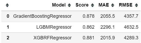
 pd.DataFrame(score, columns=['Model', 'Score', 'MAE', 'RMSE'])

Hyperparameter tuning

Let's adjust some algorithm parameters, such as tree depth, estimated value, learning rate, etc., and check the accuracy of the model. Manually trying different combinations of parameter values is time-consuming. Scikit learn's GridSearchCV automatically performs this process and calculates the optimized values of these parameters. I have applied GridSearch to the above three algorithms. Here is an example of XGBoost:

from sklearn.model_selection import GridSearchCV

param_grid = {'n_estimators': [100, 80, 60, 55, 51, 45],  
              'max_depth': [7, 8],
              'reg_lambda' :[0.26, 0.25, 0.2]
             }
                
grid = GridSearchCV(xg.XGBRFRegressor(), param_grid, refit = True, verbose = 3, n_jobs=-1) #
regr_trans = TransformedTargetRegressor(regressor=grid, transformer=QuantileTransformer(output_distribution='normal'))

# fitting the model for grid search 
grid_result=regr_trans.fit(X_train, y_train)
best_params=grid_result.regressor_.best_params_
print(best_params)

#using best params to create and fit model
best_model = xg.XGBRFRegressor(max_depth=best_params["max_depth"], n_estimators=best_params["n_estimators"], reg_lambda=best_params["reg_lambda"])
regr_trans = TransformedTargetRegressor(regressor=best_model, transformer=QuantileTransformer(output_distribution='normal'))
regr_trans.fit(X_train, y_train)
yhat = regr_trans.predict(X_test)

#evaluate metrics
r2_score(y_test, yhat), mean_absolute_error(y_test, yhat), np.sqrt(mean_squared_error(y_test, yhat))

Once we get the optimal values of the parameters, we will use these values to run all three models again.

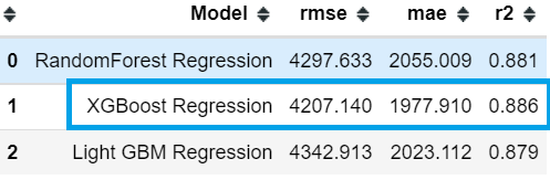
This looks much better! We have been able to improve our accuracy - XGBoost gives a score of 88.6%, with relatively few errors

The distribution and residual diagram confirm that there is a good overlap between the predicted cost and the actual cost. However, some predicted values are far beyond the x-axis, which makes our root mean square error higher. We can reduce this by increasing data points (i.e. collecting more data).

Now we are ready to deploy this model to the production environment and test it on unknown data.

In short, the key points to improve the accuracy of my model

• Create simple new features
• Convert target variable
• Clustering common data points
• Using enhanced algorithms
• Hyperparameter tuning

You can find my notebook here. Not all methods apply to your model. Choose the best solution for you:)

https://github.com/sacharya225/data-expts/tree/master/Health%20Insurance%20Cost%20Prediction

Author: Shwetha Acharya

Deep hub translation group