Introduction to HugeCTR
The large-scale sparse training based on parameter server architecture can be said that there has been no new change and progress for several years until the emergence of Baidu's aibox paper and the open source of hugectr developed by nvidia. Finally, we can see that the parameter server architecture has taken another step forward. It can be predicted that such a heterogeneous training architecture, compared with the previous pure CPU method, will have further room for improvement with the emergence of more high-performance hardware and new training optimization. I hope you can leave a message to discuss any problems and make progress together.
Related code base links: https://github.com/NVIDIA/HugeCTR/
hugectr is a GPU distributed training framework developed by nvidia. It mainly aims at recommending ctr scenarios and supports distributed training and evaluation of large-scale sparse parameters.
hugectr is a training framework based on parameter server architecture. Its main highlight is that it has a parameter server based on GPU video memory (generally speaking, there is a hashmap in GPU video memory to store parameters). In this way, during GPU training, parameters can be copied directly from GPU or communicated by GPU, which greatly accelerates parameter communication (pull and push), Because the parameter communication no longer passes through the CPU.
Of course, this also raises several questions. You might as well think about it first:
(1) We know that hashmap usually rehash when its size is close to a certain threshold. For the parameter server, with continuous training, the parameters stored in the parameter server may also increase. Especially at the beginning of training, the size of hashmap increases rapidly. If rehash is frequent or new key s are created, Then there will be frequent GPU video memory application release and copy, which will greatly affect the performance.
(2) GPU is one more step in the process of copying data from CPU to GPU. If no improvement is made, will the computing speed be faster than that of additional data copies?
(3) For large-scale sparse parameters, the scale of our key is one billion. If value (i.e. embedding vector) is a 32-dimensional float vector, if we use adam optimizer, then the optimizer state is 32 * 3 = 96 dimensions. The total parameter scale is greater than 300G. Can we put it all in video memory?
These questions will be answered step by step in the later process. Next, let's take a look at the overall architecture.
Overall architecture

Training process: first, the reader reads batch from the dataset_ Size (e.g. 32), analyze the original data, get the input spark key, deny vector, label, etc., pull the corresponding embedding vector from the parameter server (hereinafter referred to as ps, i.e. parameter server) according to the spark key, and then input it into the deep learning neural network for forward-backward calculation, The parameter gradient obtained by reverse calculation is push ed to ps, and ps updates the parameters according to the gradient.
The training process can be considered as data parallelism + model parallelism. Data parallelism is mainly reflected in that each GPU card reads different data for training at the same time, while model training is mainly reflected in that the sparse parameters are stored on multiple nodes, and each node allocates some parameters.
We know that in ctr scenarios, the size of the spark parameter is usually large, ranging from tens of millions to trillions. The deny parameter (the weight in the network) is usually small, and the memory occupied is only a few MB to tens of MB. Therefore, the access to the spark parameter needs to be well designed. There are two ways to store spark in hugectr: local and distribute.
Let's first look at the local mode: the parameters of a slot will only be on one GPU card. After checking the embedding, because we have obtained all the embedding of the slot, we can do GPU multi card communication after pooling, which can reduce the traffic. (slot here means feature type, which can also be called field)

For example, we have 4 GPU cards for stand-alone training and 8 slots: slot 0 to slot 7. In the local mode, GPU0 stores slot0 and slot1, GPU1 stores slot2 and slot3, GPU2 stores slot4 and slot5, and GPU3 stores slot6 and slot7.
For the distribution mode, some parameters of all slot s will be stored on each GPU. As for how to allocate a parameter to which GPU, you can use the hash method.
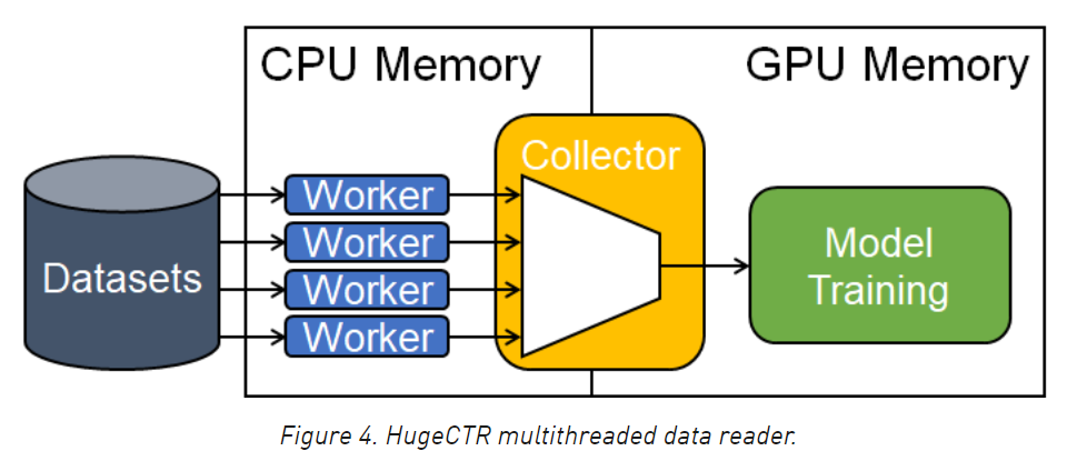
The following figure shows the process of reading data from multithreading, copying data from CPU to GPU and training. The worker in the figure actually refers to reader. Multiple readers parse the data of dataset at the same time, and then the collector module copies the data to GPU. The worker, collector and training in the figure are connected through pipelines. Each part is independent of each other and runs in different threads at the same time.
The following figure is a specific example of pipeline. Each color represents one-stage pipeline, with a total of three-stage pipeline. After the first level parses batch0, it is thrown to the second level for copying to the GPU. At this time, the first level continues to parse batch1. While batch0 is training, what it is doing at the same time is copying batch1 to GPU.
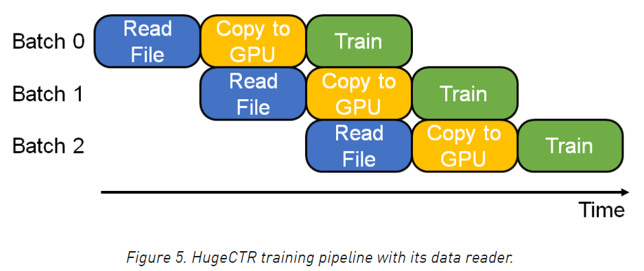
It should be noted that the time of pipelines at all levels in the above figure is equal by default, but the actual situation is generally not so coincidental. Therefore, it is generally necessary to flexibly adjust the number of threads of pipelines at all levels to match the speed of pipelines at all levels. For example, readfile has 10 threads, copy has 5 threads, and training has 8 threads. In addition, the above is actually looking at the pipeline vertically. If looking horizontally, each batch is doing readfile copy train independently of each other.
Have you found that the pipeline here answers the second question at the beginning.
Code reading
I like to look at the code from top to bottom, so that I can not only master the whole process of operation at the beginning, but also look at the details later. In addition, I didn't get too many subheadings. Just look down in order.
Let's first look at the example in readme, which is an example of calling python api. Like the common deep learning framework, hugectr is divided into python side and c + + side. python encapsulates the user api and c + + implements the underlying training logic.
   # train.py
   import sys
   import hugectr
   from mpi4py import MPI
   def train(json_config_file):
     solver_config = hugectr.solver_parser_helper(batchsize = 16384,
                                                  batchsize_eval = 16384,
                                                  vvgpu = [[0,1,2,3,4,5,6,7]],
                                                  repeat_dataset = True)
     sess = hugectr.Session(solver_config, json_config_file)
     sess.start_data_reading()
     for i in range(10000):
       sess.train()
       if (i % 100 == 0):
         loss = sess.get_current_loss()
         print("[HUGECTR][INFO] iter: {}; loss: {}".format(i, loss))
   if __name__ == "__main__":
     json_config_file = sys.argv[1]
     train(json_config_file)
In addition, if you observe the api here, you will find that it looks very similar to the tensorflow stand-alone api. Indeed, one goal of the distributed framework is to use it as easily as writing stand-alone programs, that is, the so-called "ease of use".
Solver here_ Config is to transfer various training configurations into hugectr, and session is to encapsulate the distributed training logic, start_data_reading literally means to start the asynchronous thread of readfile above, that is, the first level pipeline. Next is train, and then print oss.
As mentioned earlier, the advantage of looking at the code from the top down is that it can be targeted to the details. Let's focus on the key point first, that is, sess train.
For the connection between python and c + +, you can use the pybind library. The "bridge" of the connection is defined in pybind/session_wrapper.hpp in this file:
void SessionPybind(pybind11::module &m) {
  pybind11::class_<HugeCTR::Session, std::shared_ptr<HugeCTR::Session>>(m, "Session")
      .def(pybind11::init<const SolverParser &, const std::string &, bool, const std::string>(),
           pybind11::arg("solver_config"), pybind11::arg("config_file"),
           pybind11::arg("use_model_oversubscriber") = false,
           pybind11::arg("temp_embedding_dir") = std::string())
      .def("train", &HugeCTR::Session::train)
      .def("eval", &HugeCTR::Session::eval)
      .def("start_data_reading", &HugeCTR::Session::start_data_reading)
      ....
Call sess. In python Train corresponds to HugeCTR::Session::train of c + +. Let's take a look at this function. I added some comments:
bool Session::train() {
    // Judge whether the reader is started. If you start training without starting, an error will be reported
    if (train_data_reader_->is_started() == false) {
      CK_THROW_(xxxx);
    }
    // Wait for the reader to read the data of at least one batchsize
    long long current_batchsize = 0;
    while ((current_batchsize = train_data_reader_->read_a_batch_to_device_delay_release()) &&
           (current_batchsize < train_data_reader_->get_full_batchsize())) {
      // Tell the reader to start parsing data by setting flag: READY_TO_WRITE
      train_data_reader_->ready_to_collect();
    }
    // If the data cannot be read, that is, there is no data to train, return directly
    if (!current_batchsize) {
      return false;
    }
    // After the reader parses the data of a batch, the flag will be set to READY_TO_READ
    // Read above_ a_ batch_ to_ device_ delay_ Release takes the data from the reader,
    // And asynchronously copying to GPU,
    // Call ready_to_collect, first sync the asynchronous copy above, and then let the reader continue to parse the next batch
    train_data_reader_->ready_to_collect();
    // Check embedding from ps and make sum or avg
    for (auto& one_embedding : embeddings_) {
      one_embedding->forward(true);
    }
    // The logic here looks a little messy, that is, multi card data parallel training,
    // A network has several copies of gpu cards, which is why the size of networks is greater than 1.
    if (networks_.size() > 1) {
      // Single machine multi card or multi machine multi card
      // execute dense forward and backward with multi-cpu threads
      #pragma omp parallel num_threads(networks_.size())
      {
        // Forward and reverse of dense network
        size_t id = omp_get_thread_num();
        long long current_batchsize_per_device =
            train_data_reader_->get_current_batchsize_per_device(id);
        networks_[id]->train(current_batchsize_per_device);
        // Gradient of exchanging dense parameters between multi cards
        networks_[id]->exchange_wgrad();
        // Update the deny parameter
        networks_[id]->update_params();
      }
    } else if (resource_manager_->get_global_gpu_count() > 1) {
      // Multi machine single card
      long long current_batchsize_per_device =
          train_data_reader_->get_current_batchsize_per_device(0);
      networks_[0]->train(current_batchsize_per_device);
      networks_[0]->exchange_wgrad();
      networks_[0]->update_params();
    } else {
      // Single card
      long long current_batchsize_per_device =
          train_data_reader_->get_current_batchsize_per_device(0);
      networks_[0]->train(current_batchsize_per_device);
      networks_[0]->update_params();
    }
    // Reverse of embedding
    for (auto& one_embedding : embeddings_) {
      one_embedding->backward();
      // Update spark parameter
      one_embedding->update_params();
    }
    return true;
}
See here, the general process of training is basically clear. Next, let's continue to look at reader, embedding, parameter storage and communication. First, it is necessary to look at initialization.
The initialization code of HugeCTR::Session is as follows:
parser.create_pipeline(
    train_data_reader_, evaluate_data_reader_,
    embeddings_, networks_, resource_manager_);
#pragma omp parallel num_threads(networks_.size())
{
  size_t id = omp_get_thread_num();
  networks_[id]->initialize();
  if (solver_config.use_algorithm_search) {
    networks_[id]->search_algorithm();
  }
  CK_CUDA_THROW_(cudaStreamSynchronize(
      resource_manager_->get_local_gpu(id)->get_stream()));
}
init_or_load_params_for_dense_(solver_config.model_file);
init_or_load_params_for_sparse_(solver_config.embedding_files);
load_opt_states_for_sparse_(solver_config.sparse_opt_states_files);
load_opt_states_for_dense_(solver_config.dense_opt_states_file);
It is divided into the following steps:
(1) Create a three-stage pipeline, i.e. create_pipeline
(2) Initialize network
(3) Initialization parameters and corresponding optimizer status
The more important part is to create a three-stage pipeline. Let's take a look at create_ Implementation of pipeline (function parameters are ignored first):
// create reader
create_datareader<TypeKey>()(...);
// create embedding
for (unsigned int i = 1; i < j_layers_array.size(); i++) {
  // Each layer of network configuration is from bottom to top, so as long as non embedded layers are encountered,
  // You don't have to check the back layer
  const nlohmann::json& j = j_layers_array[i];
  auto embedding_name = get_value_from_json<std::string>(j, "type");
  Embedding_t embedding_type;
  if (!find_item_in_map(embedding_type, embedding_name, EMBEDDING_TYPE_MAP)) {
    break;
  }
  create_embedding<TypeKey, float>()(...);
}
// create network: create a network copy for each GPU card
for (size_t i = 0; i < resource_manager->get_local_gpu_count(); i++) {
  network.emplace_back(Network::create_network(...));
}
You can see create_pipeline mainly includes three steps: create_datareader,create_embedding,create_network
Let's start with create_ What does datareader do: create a train_data_reader and an evaluate_data_reader, that is, one for training and one for evaluation. Then they created their own workergroups.
DataReader<TypeKey>* data_reader_tk = new DataReader<TypeKey>(...);
train_data_reader.reset(data_reader_tk);
DataReader<TypeKey>* data_reader_eval_tk = new DataReader<TypeKey>(...);
evaluate_data_reader.reset(data_reader_eval_tk);

train_data_reader->create_drwg_norm(source_data, check_type, repeat_dataset_);
evaluate_data_reader->create_drwg_norm(eval_source, check_type, repeat_dataset_);
  void create_drwg_norm(std::string file_name, Check_t check_type,
                        bool start_reading_from_beginning = true) override {
    source_type_ = SourceType_t::FileList;
    worker_group_.reset(new DataReaderWorkerGroupNorm<TypeKey>(
        csr_heap_, file_name, repeat_, check_type, params_, start_reading_from_beginning));
    file_name_ = file_name;
  }

// The constructor of DataReaderWorkerGroupNorm is mainly used for the following functions to create DataReaderWorker
for (int i = 0; i < NumThreads; i++) {
  std::shared_ptr<IDataReaderWorker> data_reader(new DataReaderWorker<TypeKey>(
          i, NumThreads, csr_heap, file_list, max_feature_num_per_sample, repeat, check_type, params));
  data_readers_.push_back(data_reader);
}
// Then multiple threads are created. Each thread corresponds to a reader and executes the following logic
while (*p_loop_flag) {
  data_reader->read_a_batch();
}
Well, see here, there are two classes DataReader and DataReaderWorkerGroupNorm. It is necessary to look at the details of these two classes to clarify the data reading.
Let's first look at the important functions and variables in DataReader:
template <typename TypeKey>
class DataReader : public IDataReader {
  std::shared_ptr<HeapEx<CSRChunk<TypeKey>>> csr_heap_;
  std::shared_ptr<DataCollector<TypeKey>> data_collector_;
  std::shared_ptr<DataReaderWorkerGroup> worker_group_;
  //There are also various tensors: labels_ tensors_, dense_tensors_, row_offsets_tensors_, value_tensors_ etc.
  DataReader(...) {
    // Initialize heap. This class is described later
    csr_heap_.reset(new HeapEx<CSRChunk<TypeKey>>(...));
    // Initialize a buffer for each GPU
    std::vector<std::shared_ptr<GeneralBuffer2<CudaAllocator>>> buffs;
    for (size_t i = 0; i < local_gpu_count; i++) {
      buffs.push_back(GeneralBuffer2<CudaAllocator>::create());
    }
    // create label and dense tensor
    size_t batch_size_per_device = batchsize_ / total_gpu_count;
    for (size_t i = 0; i < local_gpu_count; i++) {
      // Tensor2 does not hold memory or video memory. It is in buffs
      {
        Tensor2<float> tensor;
        buffs[i]->reserve({batch_size_per_device, label_dim_}, &tensor);
        label_tensors_.push_back(tensor);
      }
      {
        Tensor2<float> tensor;
        buffs[i]->reserve({batch_size_per_device, dense_dim_}, &tensor);
        dense_tensors_.push_back(tensor.shrink());
      }
    }
    ...
    // Here is another DataCollector class
    data_collector_.reset(new DataCollector<TypeKey>(...);
    data_collector_->start();
    // buffs allocates video memory on each GPU
    for (size_t i = 0; i < local_gpu_count; i++) {
      CudaDeviceContext context(resource_manager_->get_local_gpu(i)->get_device_id());
      buffs[i]->allocate();
    }
  }
Introduce the above classes in detail:
(1) CSR: a storage format used to compress sparse matrices. Examples are as follows
If there is such a set of data
 *   4,5,1,2
 *   3,5,1
 *   3,2
 use CSR Can be expressed as
  row offset: 0,4,7,9
  value: 4,5,1,2,3,5,1,3,2
Since CSR here is used to store the spark keys in a slot, column index is actually missing, because the spark keys in a slot can be stored directly in sequence. CSR can refer to this article article . It is always reminiscent of Baidu paddle's lodsensor.
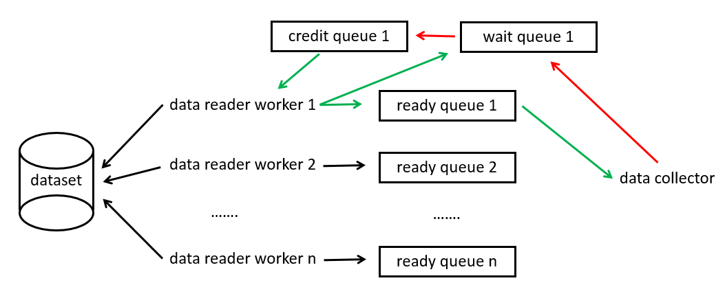
(2) HeapEx: three queues are maintained for each data parsing thread: ready queue, wait queue and credit queue. The elements in the queue are CSR storage. When the credit queue is not empty, it means that there is an idle CSR that can be used to store the parsed data.
- Parsing data (multithreading): the current thread will only operate its own queue. After a free CSR is taken out from the credit queue, it will be stuffed into the wait queue at the same time. After the data is parsed and saved into the CSR, it will be removed from the wait queue and stuffed into the ready queue (the reason why there is one more step in the wait queue is mainly to record the CSR and then stuffed into the ready queue).
- Read data (single thread): fetch data from the above multiple queues. There is a variable count in HeapEx, which records the data obtained from the ready queue of the data parsing thread of the index last time. The next time the data is retrieved, it will be traversed from the ready queue of the index, that is, "polling", and the data will be returned to the index. Return or return to the credit queue and remove it from the ready queue. After angelica is returned successfully, count + +. (why not remove the data from the ready queue when fetching data? Because fetching data is a single thread, it is possible to do so)
(3) Datareader worker: the above thread for parsing data.
(4) Data collector: it is the above data reading thread. Copy data from CSR to GPU. It will start a thread and continuously execute the following functions:
template <typename TypeKey>
void DataCollector<TypeKey>::collect_() {
  std::unique_lock<std::mutex> lock(stat_mtx_);
  CSRChunk<TypeKey>* chunk_tmp = csr_heap_->checkout_data_chunk();
  while (stat_ != READY_TO_WRITE && stat_ != STOP) {
    usleep(2);
  }
  ...
  cudaMemcpyAsync Make a copy
  ...
  cudaStreamSynchronize
  ...
  csr_heap_->return_free_chunk();
  stat_ = READY_TO_READ;
Check out here_ data_ Chunk takes a CSR from a queue and calls return after copying_ free_ Chunk return.
In order to express the process clearly, I drew a simple diagram. The green line is data production and consumption, and the red line is data return. When the data reader worker obtains the idle CSR, it parses the data, fills it in and puts it into the ready queue. When the data collector finds that there is an available CSR, it copies it to the GPU and returns it to the CSR. It can be said that data reader, worker and data collector are independent of each other, and they are connected through the queue for storing data.
There are also some details worth noting:
(1) hugectr also implements two kinds of data reader worker s. One is DataReaderWorkerRaw. The data it reads is directly mapped to memory through mmap. Another is DataReaderWorkerGroup, which reads parquet format files.
(2) Details of data reader worker parsing data into CSR:
// Get returns yes_ batch size of training configuration
for (i = 0; i < csr_chunk->get_batchsize(); i++) {
  // Deny input
  {
    // label_ dense_ The size of buffers is the number of gpu cards in the current node
    // buffer_id is the card on which the sample falls
    int buffer_id = i / (csr_chunk->get_batchsize() / label_dense_buffers.size());
    // local_id is the offset of this sample on the current card
    int local_id = i % (csr_chunk->get_batchsize() / label_dense_buffers.size());
    // Copy: copy from the buffer of parsing data to CSR
    float* ptr = label_dense_buffers[buffer_id].get_ptr();
    for (int j = 0; j < label_dense_dim; j++) {
        ptr[local_id * label_dense_dim + j] = label_dense[j];  // row major for label buffer
    }
  }
  // Spark input
  for (auto& param : params_) {
    for (int k = 0; k < param.slot_num; k++) {
      // Reading data is omitted
      ...
      // The following code is very helpful to understand the two storage methods of embedding
      if (param.type == DataReaderSparse_t::Distributed) {
        // All slot s will be stored on each card of all nodes
        for (int dev_id = 0; dev_id < csr_chunk->get_num_devices(); dev_id++) {
          csr_chunk->get_csr_buffer(param_id, dev_id).new_row();
        }
        // This is to judge which card the slot key should be stored on
        for (int j = 0; j < nnz; j++) {
          int dev_id = feature_ids_[j] % csr_chunk->get_num_devices();
          dev_id = std::abs(dev_id);
          T local_id = feature_ids_[j];
          csr_chunk->get_csr_buffer(param_id, dev_id).push_back(local_id);
        }
      } else if (param.type == DataReaderSparse_t::Localized) {
        // A slot can only exist on one card
        int dev_id = k % csr_chunk->get_num_devices();
        csr_chunk->get_csr_buffer(param_id, dev_id).new_row();
        for (int j = 0; j < nnz; j++) {
          T local_id = feature_ids_[j];
          csr_chunk->get_csr_buffer(param_id, dev_id).push_back(local_id);
        }
      }
    }
  }
}
(3) Details of data collector copying data:
  // total_device_count the sum of GPUs of all nodes
  for (int ix = 0; ix < total_device_count; ix++) {
    int i =
        ((id_ == 0 && !reverse_) || (id_ == 1 && reverse_)) ? ix : (total_device_count - 1 - ix);
    int pid = resource_manager_->get_process_id_from_gpu_global_id(i);
    int label_copy_num = (label_dense_buffers[0]).get_num_elements();
    if (pid == resource_manager_->get_process_id()) {
      ...
      for (int j = 0; j < num_params; j++) {
        // I * num here_ Params + J takes the global offset
        unsigned int nnz = csr_cpu_buffers[i * num_params + j]
                               .get_row_offset_tensor()
                               .get_ptr()[csr_cpu_buffers[i * num_params + j].get_num_rows()];
        // cudaMemcpyAsync asynchronous copy
    }
We found that all nodes will parse all data! When copying, only the data belonging to this node will be copied. The performance of this implementation is questionable for a large amount of data. The bandwidth may not be enough, and a large amount of useless data will be parsed.
On the one hand, only the spark keys belonging to the gpu will be reserved during data copying. On the other hand, only the spark keys belonging to the node will be stored in the gpu. In other words, there is no need to communicate between nodes during spark pull and push. Of course, the subsequent communication between nodes still needs to be done. The data is assembled into a complete batch for forward and reverse calculation. After obtaining the gradient, the gradient average between nodes is done. This will be expanded in detail at create embedding.
In fact, the above data reader, worker and data collector are the first and second stage pipelines in the figure at the beginning of this article. Next, let's look at create in the third stage pipeline_ Embedding part.
When creating embedding initialization, we should pay most attention to how to save parameters. Before that, let's take a look at the network configuration and how to organize embedding. Here, take deepfm as an example. First, let's take a look at the input layer
      "dense": {
        "top": "dense",
        "dense_dim": 13
      },
      "sparse": [
        {
          "top": "data1",
          "type": "DistributedSlot",
          "max_feature_num_per_sample": 30,
          "slot_num": 26
	    }
      ]
The deny input is the fm input of deepfm. Spark is the deep input of deepfm and contains 26 slot s. Let's look at the definition of embedding layer, max_vocabulary_size_per_gpu is the maximum number of spark keys on a gpu card_ vec_ Size is the embedding vector dimension, and combiner indicates whether it is sum or avg after checking embedding for pooling.
    {
      "name": "sparse_embedding1",
      "type": "DistributedSlotSparseEmbeddingHash",
      "bottom": "data1",
      "top": "sparse_embedding1",
      "sparse_embedding_hparam": {
        "max_vocabulary_size_per_gpu": 1447751,
        "embedding_vec_size": 11,
        "combiner": 0
      }
    }
hugectr has two kinds of embedding: distributed slotsparseembeddinghash and localized slotsparseembeddinghash. Let's look at it one by one.
At a glance, the code created by hashmap is the same:
// Note that the value type of hash table is a size_t. This is the offset of embedding in storage
using NvHashTable = HashTable<TypeHashKey, size_t>;
// This is the definition of hashmap. It is found that there is a vector outside. We need to find out what each element of the vector is
std::vector<std::shared_ptr<NvHashTable>> hash_tables_;
// The original vector size is the number of local GPUs, that is, each gpu card corresponds to a hash table
hash_tables_.resize(Base::get_resource_manager().get_local_gpu_count());
// The maximum number of elements contained in the hash table is fixed to Max in advance_ vocabulary_ size_ per_ gpu_
#pragma omp parallel num_threads(Base::get_resource_manager().get_local_gpu_count())
{
  size_t id = omp_get_thread_num();
  CudaDeviceContext context(Base::get_local_gpu(id).get_device_id());
  // construct HashTable object: used to store hash table <key, value_index>
  hash_tables_[id].reset(new NvHashTable(max_vocabulary_size_per_gpu_));
  Base::get_buffer(id)->allocate();
}
Here we can answer the first question at the beginning. The answer is very simple and rough. It is to fix the size of the hash table in advance.
In fact, for large-scale sparsity, the supported parameter scale will not be very large, just like the 100 million level calculated in the third question at the beginning has to be 300G. Therefore, the parameter scale supported by hugectr will be greatly limited due to such design.
Is the third problem unsolvable? In fact, it is not. Baidu's aibox does not have such restrictions, because it adopts multi-level ps (ssd+mem+gpu), and the size of gpu ps will dynamically create hashmap s of different sizes with the number of key s of incremental data currently trained. Aibox won't start here for the time being. I'll write an article about it later
Continue to look at the HashTable class
template <typename KeyType, typename ValType>
class HashTable {
  // Find the key. If the key is not in the table, insert it
  void get_insert(const KeyType* d_keys, ValType* d_vals, size_t len, cudaStream_t stream);
  // Find key
  void get(const KeyType* d_keys, ValType* d_vals, size_t len, cudaStream_t stream) const;
  // dump all the kv in the table
  void dump(KeyType* d_key, ValType* d_val, size_t* d_dump_counter, cudaStream_t stream) const;
  HashTableContainer<KeyType, ValType>* container_
Let's take another look at HashTableContainer, which inherits concurrent_unordered_map this class
template <typename KeyType, typename ValType>
class HashTableContainer
    : public concurrent_unordered_map<KeyType, ValType, std::numeric_limits<KeyType>::max()> {
 public:
  HashTableContainer(size_t capacity)
      : concurrent_unordered_map<KeyType, ValType, std::numeric_limits<KeyType>::max()>(
            capacity, std::numeric_limits<ValType>::max()) {}
};
concurrent_unordered_map is a fixed size map in video memory. It supports concurrent insert, but does not support concurrent insert and get. Because hugectr training is synchronous training, there will only be get when pulling and insert when pushing, and it will not do pull and push at the same time_ unordered_ The map meets the requirements.
First take a look at its get function:
// __ forceinline__  Force specified as inline function
// __ host__ __device__  This function will be compiled for both host side and device side
__forceinline__ __host__ __device__ const_iterator find(const key_type& k) const {
    // Hash key
    size_type key_hash = m_hf(k);
    // An index mapped to table
    size_type hash_tbl_idx = key_hash % m_hashtbl_size;
    value_type* begin_ptr = 0;
    size_type counter = 0;
    while (0 == begin_ptr) {
      value_type* tmp_ptr = m_hashtbl_values + hash_tbl_idx;
      const key_type tmp_val = tmp_ptr->first;
      // Found this key
      if (m_equal(k, tmp_val)) {
        begin_ptr = tmp_ptr;
        break;
      }
      // This position is empty, or the table is not found after searching
      if (m_equal(unused_key, tmp_val) || counter > m_hashtbl_size) {
        begin_ptr = m_hashtbl_values + m_hashtbl_size;
        break;
      }
      hash_tbl_idx = (hash_tbl_idx + 1) % m_hashtbl_size;
      ++counter;
    }
    return const_iterator(m_hashtbl_values, m_hashtbl_values + m_hashtbl_size, begin_ptr);
  }
It can be seen that when you get a key, if you insert the key, you may still not get it, or get the wrong value (you get the value when the insert is modifying the value), or the old value.
Take another look at insert. Its main process is as follows
const key_type insert_key = k;
bool insert_success = false;
size_type counter = 0;
while (false == insert_success) {
  // Hash table full
  if (counter++ >= hashtbl_size) {
    return end();
  }
  key_type& existing_key = current_hash_bucket->first;
  volatile mapped_type& existing_value = current_hash_bucket->second;
  // existing_key == unused_key, insert_key will be assigned to existing_key, because this position is empty.
  // existing_key == insert_key, there is already this key in this position,
  // If existing at this time_ value == m_ unused_ Element indicates that other threads are insert ing and have not had time to modify existing_value
  const key_type old_key = atomicCAS(&existing_key, unused_key, insert_key);
  if (keys_equal(unused_key, old_key)) {
    existing_value = (mapped_type)(atomicAdd(value_counter, 1));
    break;
  } else if (keys_equal(insert_key, old_key)) {
    while (existing_value == m_unused_element) { }
    break;
  }
  // This position is occupied by other key s. Continue to traverse back
  current_index = (current_index + 1) % hashtbl_size;
  current_hash_bucket = &(hashtbl_values[current_index]);
}
return iterator(m_hashtbl_values, m_hashtbl_values + hashtbl_size, current
atomicCAS functions refer to this article article.
Two embedding s:
(1)DistributedSlotSparseEmbeddingHash
void forward(bool is_train) override {
  // Read data from input_buffers_ -> look up -> write to output_tensors
  CudaDeviceContext context;
  for (size_t i = 0; i < Base::get_resource_manager().get_local_gpu_count(); i++) {
    context.set_device(Base::get_local_gpu(i).get_device_id());
    functors_.forward_per_gpu(..., Base::get_local_gpu(i).get_stream());
  }
  // do reduce scatter
  size_t recv_count = Base::get_batch_size_per_gpu(is_train) *
                      Base::get_slot_num() *
                      Base::get_embedding_vec_size();
  functors_.reduce_scatter(recv_count, embedding_feature_tensors_,
                           Base::get_output_tensors(is_train), Base::get_resource_manager());
  // scale for combiner=mean after reduction
  if (Base::get_combiner() == 1) {
    size_t send_count = Base::get_batch_size(is_train) * Base::get_slot_num() + 1;
    functors_.all_reduce(send_count, Base::get_row_offsets_tensors(is_train),
                         row_offset_allreduce_tensors_, Base::get_resource_manager());
    // do average
    functors_.forward_scale(Base::get_batch_size(is_train), Base::get_slot_num(),
                            Base::get_embedding_vec_size(), row_offset_allreduce_tensors_,
                            Base::get_output_tensors(is_train), Base::get_resource_manager());
  }
  return;
}
Let's first look at forward. First, look up from the hashmap of the current gpu, that is, functions_ forward_ per_ gpu, there is no need for inter node communication at this time, because the key s of the data corresponding to the current gpu are in the current gpu.
Then I did reduce scatter. For this communication, please refer to this article Official documents
Each slot size is a piece of data in each slot, but each slot size is a piece of data in each slot. After the reduce scatter, the data is complete, and each gpu is divided into a part of the complete data.
Let's assume that there are two GPUs in total, the batch size is 2, and there are three slot s in total. Then the above process is as follows:

If you want to do mean pooling, you need to do all reduce again to get the total number of key s in each sample and each slot (calculate the offset in csr into allreduce to get the global offset), and then divide the embedding value by this number, that is, to find the average.
Take another look at backward
void backward() override {
  // Read dgrad from output_tensors -> compute wgrad
  // do all-gather to collect the top_grad
  size_t send_count =
      Base::get_batch_size_per_gpu(true) * Base::get_slot_num() * Base::get_embedding_vec_size();
  functors_.all_gather(send_count, Base::get_output_tensors(true), embedding_feature_tensors_,
                       Base::get_resource_manager());
  // do backward
  functors_.backward(...);
  return;
}
First, do all gather, get the gradients of all samples of the current batch for each gpu, and then update the parameters on each local gpu.
void update_params() override {
  #pragma omp parallel num_threads(Base::get_resource_manager().get_local_gpu_count())
  {
    size_t id = omp_get_thread_num();
    CudaDeviceContext context(Base::get_local_gpu(id).get_device_id());
    // accumulate times for adam optimizer
    Base::get_opt_params(id).hyperparams.adam.times++;
    // do update params operation
    functors_.update_params(...);
  }
  return;
}
Dump is divided into dump parameter and dump optimizer status. Their codes are similar. The following are dump parameters:
// dump hash table from GPUs
for (size_t id = 0; id < local_gpu_count; id++) {
  // dump key
  hash_tables[id]->dump
  // Copy to memory
  cudaMemcpyAsync(...,cudaMemcpyDeviceToHost,...)
  // dump value
  functors_.get_hash_value
  // Copy to memory
  cudaMemcpyAsync(...,cudaMemcpyDeviceToHost,...)
}
functors_.sync_all_gpus(...)
for (size_t id = 0; id < local_gpu_count; id++) {
  // Total size of parameters on each gpu
  size_t size_in_B = count[id] * (sizeof(TypeHashKey) + sizeof(float) * embedding_vec_size);
  // memcpy to file_buf
  ...
  // The rank 0 node is responsible for writing files
  if (Base::get_resource_manager().is_master_process()) {
    weight_stream.write(file_buf.get(), size_in_B);
  } else {
    // Other nodes send data to rank0 node
    MPI_Send(file_buf.get(), size_in_B, ...);
  }
}
// rank0 node receives data
if (Base::get_resource_manager().is_master_process()) {
  for (int r = 1; r < Base::get_resource_manager().get_num_process(); r++) {
    for (size_t id = 0; id < local_gpu_count; id++) {
      ...
      MPI_Recv(...);
      weight_stream.write(file_buf.get(), size_in_B);
    }
  }
}
// Release gpu video memory
cudaFree
Note that during dump, both parameters and optimizer status need to be passed through MPI_SEND to a node. When the parameter scale is relatively large, node 0 will become a bottleneck. Instead of each node dump's own parameters, you can also organize the parameters by slice.
During load, each node will load all model files, and then judge whether each key belongs to itself:
TypeHashKey key = key_ptr[...];
size_t gid = key % global_gpu_count; // global GPU ID
int dst_rank = get_process_id_from_gpu_global_id(gid);  // node id
if (my_rank == dst_rank) {
    memcpy(...)
} else {
  continue;
}
(2)LocalizedSlotSparseEmbeddingHash
void forward(bool is_train) override {
    CudaDeviceContext context;
    for (size_t i = 0; i < Base::get_resource_manager().get_local_gpu_count(); i++) {
      context.set_device(Base::get_local_gpu(i).get_device_id());  // set device
      functors_.forward_per_gpu(...);
    }
    functors_.all2all_forward(...);
    // reorder: reorganize the received data buffer
    functors_.forward_reorder(...);
    // Save the slot id corresponding to each spark parameter pair
    functors_.store_slot_id(...);
    return;
}
all2all_ The process of forward is as follows:
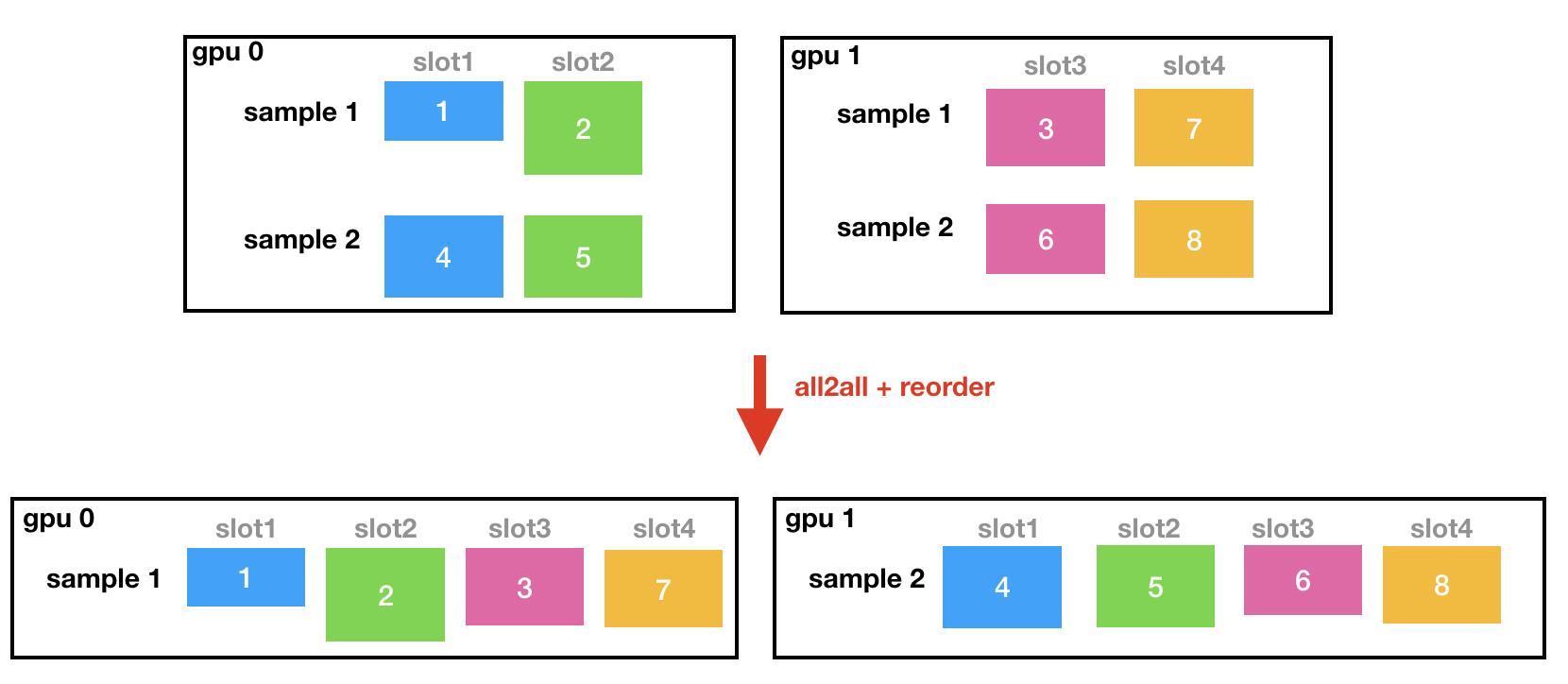
The reorder process can be understood as follows:

The reason for saving the slot id corresponding to the parameter is that different slots are stored on each gpu. When loading, you need to know which slot parameters to load.
create_network is mainly to create various layers of neural network.
After performing the forward reverse, the gradient will be averaged between multiple cards first, and then the deny parameter will be updated.
void Network::exchange_wgrad() {
  CudaDeviceContext context(get_device_id());
  ncclAllReduce((const void*)wgrad_tensor_.get_ptr(),
                (void*)wgrad_tensor_.get_ptr(), wgrad_tensor_.get_num_elements(),
                ncclFloat, ncclSum, gpu_resource_->get_nccl(),
                pu_resource_->get_stream()));
}
At this point, the whole training process should be clear. Let's talk about hybrid accuracy training again. Hugectr mentioned hybrid accuracy training in the Highlighted features in the official introduction. In hugectr, the parameter storage of embedding layer is full precision float32. If mixed is configured_ Precision, then the embedded layer optimizer state uses half precision fp16, and its output is also half precision fp16, and other dense layers that support fp16 calculation will also use fp16 calculation. You can read this article article.
After you have a general understanding of hugectr, you can run it again hugectr An example of the official code base.
After a brief summary of the advantages and disadvantages of gectr Code:
advantage:
- Large batch training / complex model training, sparse parameters are distributed on multiple GPUs, and worker and ps are in the same process. Support mixed accuracy training.
- The embedding table is stored in the gpu, and the sparse parameter communication is faster than that of the cpu. Embedding after the lookup of this node, do sum/embedding first to reduce the traffic. The dense parameter is also communicated through gpu.
- Three stage pipeline, hidden data time: parsing data (data reader worker), copying data to gpu (collector), training (forward and reverse + updating parameters).
Disadvantages:
- Each node downloads and parses the full amount of data. When the amount of data is large, the bandwidth will become a bottleneck.
- In dump model, only node 0 is executed. When the number of parameters is large, node 0 will become a bottleneck.
- After lookup, samples need to be exchanged between nodes: both distributed slotsparseembeddinghash and localized slotsparseembeddinghash need communication exchange samples. There is no obvious difference and advantage between the two modes.
- The video memory of the parameter server needs to be allocated in advance, and the size is fixed, which is not suitable for scenes with a large number of parameters.