Pre knowledge of image enhancement

Image enhancement is a very important image preprocessing process in image pattern recognition. The purpose of image enhancement is to enhance the information conducive to pattern recognition, suppress the information unfavorable to pattern recognition, expand the difference between different object features in the image, and lay a good foundation for image information extraction and recognition. According to different implementation methods, image enhancement can be divided into point enhancement, spatial enhancement and frequency domain enhancement.

1. Point enhancement Point enhancement mainly refers to image gray transformation and geometric transformation. Gray scale transformation of image is also called point operation, contrast enhancement or contrast stretching. It is an important part of image digitization software and image display software. Gray transformation is a simple and important technology, which allows users to change the gray range occupied by image data. An input image will generate a new output image after gray transformation. The gray value of the corresponding output pixel is determined by the gray value of the input pixel. Gray scale transformation does not change the spatial relationship in the image. Image geometric transformation is another basic transformation in image processing. It usually includes image translation, image mirror transformation, image scaling and image rotation. Through the geometric transformation of the image, the most basic coordinate transformation and scaling functions of the image can be realized.

2. Airspace enhancement The spatial information of the image can reflect the position, shape, size and other characteristics of the object in the image, which can be described by a certain physical mode. For example, the edge contour of an object generally has high-frequency characteristics due to the drastic change of gray value, while the interior of a relatively smooth object presents low-frequency characteristics due to the uniformity of gray value. Therefore, the high-frequency and low-frequency features of the image can be enhanced respectively as needed. The high-frequency enhancement of the image can highlight the edge contour of the object, so as to sharpen the image. For example, for face comparison and query, it is necessary to highlight the outline of the five palaces through high-frequency enhancement technology. Accordingly, enhancing the low-frequency part of the image can smooth the image, which is generally used for image noise elimination.

3. Frequency domain enhancement The spatial domain enhancement of image generally only enhances the digital image locally, while the frequency domain enhancement of image can enhance the image globally. Frequency domain enhancement technology is to filter the image in the frequency domain space of digital image, so it is necessary to transform the image from spatial domain to frequency domain, which is generally realized by Fourier transform. Spatial filtering in frequency domain can be realized by convolution as spatial filtering, so Fourier transform and convolution theory are the basis of frequency domain filtering technology.

Classification of image enhancement methods:

|Image enhancement method | implementation method| |-|-| |Processing object | gray image| ||(pseudo) color map| |-|-| |Processing strategy | global processing| ||ROI, region of interest| |-|-| |Processing method | spatial domain (point domain operation, i.e. gray transformation)| ||Spatial domain (neighborhood method, i.e. spatial filtering)| ||Frequency domain method| |-|-| |Processing purpose | image sharpening| ||Smooth denoising| ||Grayscale adjustment (contrast enhancement)|

Contrast enhancement of image enhancement methods

|Image enhancement method | implementation method| |-|-| |Gray scale transformation method | linear transformation (realized)| ||Logarithmic transformation (implemented)| ||Exponential transformation (implemented)| |-|-| |Histogram adjustment method | histogram equalization (realized)| ||Histogram matching (not implemented)|

Image contrast enhancement

|||| |-|-|-| |Image contrast enhancement | direct|| ||Indirect histogram stretching| |||Histogram equalization| ||||

Histogram Stretch 
    The histogram is adjusted by contrast stretching, so as to "expand" the difference between foreground and background gray, so as to enhance the contrast. This method can be realized by linear or nonlinear methods;Histogram equalization uses the cumulative function to "adjust" the gray value to enhance the contrast.
Histogram equalization processing
    "The central idea is to change the gray histogram of the original image from a certain gray range to a uniform distribution in all gray ranges. Histogram equalization is to stretch the image nonlinearly and redistribute the image pixel values so that the number of pixels in a certain gray range is roughly the same. Histogram equalization is to change the histogram distribution of a given image into a "uniform" distribution.

Common image enhancement

Histogram equalization

|Histogram equalization|| |-|-| |Advantages | it is very effective to process over bright and dark images (overexposed or underexposed), and depict more details| ||It is a very intuitive technology and reversible operation. If the equalization function is known, the original histogram can be restored, and the amount of calculation is small| |-|-| |Disadvantages | the processing data is random, which may reduce the signal-to-noise ratio (increase the background noise contrast and reduce the useful signal contrast)|

c language code:

#include <stdio.h>
#include <iostream>
#include "fftw3.h"
#include "string"
#include "vector"
#include <windows.h>
#include <opencv2/legacy/legacy.hpp>
#include <opencv2/nonfree/nonfree. hpp>//opencv_ Nonfree module: contains some patented algorithms, such as SIFT and SURF function source code. 
#include "opencv2/core/core.hpp"
#include "opencv2/features2d/features2d.hpp"
#include "opencv2/highgui/highgui.hpp"
#include <opencv2/nonfree/features2d.hpp>
 
using namespace cv;
using namespace std;
 
class hisEqt
{
public:
    hisEqt::hisEqt();
    hisEqt::~hisEqt();
public:
    int w;
    int h;
    int nlen;
 
    int *pHis;
    float *pdf;
 
    //=====Calculate the probability density of pixel distribution====  
    void  getPdf();
 
    //======Count the number of pixels=======  
    void getHis(unsigned char*imgdata);
 
    //==========Draw statistical distribution histogram===============  
    void drawHistogram(const float*pdf,Mat &hist1);  
 
    //===========Histogram equalization==========  
    void hisBal();
 
    //====Histogram equalized image===  
    void imgBal(unsigned char* img);
};
 
 
hisEqt::hisEqt() :nlen(0){
    pHis = new int[256 * sizeof(int)];
    memset(pHis, 0, 256 * sizeof(int));
    pdf = new float[255 * sizeof(float)];
    memset(pdf, 0, 255 * sizeof(float));
}
 
hisEqt::~hisEqt(){
    delete[]pHis;
    delete[]pdf;
}
 
 
//======Count the number of pixels=======  
void hisEqt::getHis(unsigned char*imgdata){
    for (int i = 0; i<nlen; i++)
    {
        pHis[imgdata[i]]++;
    }
}
 
 
//=====Calculate the probability density of pixel distribution====  
void hisEqt::getPdf(){
    for (int k = 0; k<256; k++)
    {
        pdf[k] = pHis[k] / float(nlen);
    }
}
 
//===========Histogram equalization==========  
void hisEqt::hisBal(){
    for (int k = 1; k<256; k++)
    {
        pdf[k] += pdf[k - 1];
    }
    for (int k = 0; k<256; k++)
    {
        pHis[k] = 255 * pdf[k];
    }
}
 
//====Histogram equalization  
void hisEqt::imgBal(unsigned char* img){
    for (int i = 0; i<nlen; i++)
    {
        img[i] = pHis[img[i]];
    }
}
 
 
void hisEqt::drawHistogram(const float *pdf, Mat& hist1){
    for (int k = 0; k<256; k++)
    {
        if (k % 2 == 0)
        {
            Point a(k, 255), b(k, 255 - pdf[k] * 2550);
            line(hist1,
                a,
                b,
                Scalar(0, 0, 255),
                1);
        }
        else
        {
            Point a(k, 255), b(k, 255 - pdf[k] * 2550);
            line(hist1,
                a,
                b,
                Scalar(0, 255, 0),
                1);
        }
    }
}
 
 
int main()
{
    Mat image = imread("Fig0651(a)(flower_no_compression).tif");
    if (!image.data)
        return -1;
 
    Mat hist2(256, 256, CV_8UC3, Scalar(0, 0, 0));
    Mat hist1(256, 256, CV_8UC3, Scalar(0, 0, 0));
 
    Mat imgOut = Mat(image.rows, image.cols, CV_8UC3, Scalar(0, 0, 0));
    vector<Mat> planes;
    int chn = image.channels();
    if (chn == 3)
    {
        split(image, planes);
    }
    while (chn)
    {
        chn--;
        unsigned char* imageData = new unsigned char[sizeof(unsigned char)*(image.cols*image.rows)];
        memcpy(imageData, planes[chn].data, planes[chn].cols*planes[chn].rows);
        hisEqt his;//Custom class
        his.nlen = image.rows*image.cols;
        his.getHis(imageData);
        his.getPdf();
 
        //  //======Draw the original histogram and save it============  
        his.drawHistogram(his.pdf, hist1);
        string pic_name = "hisline";
        pic_name = pic_name + to_string(chn);
        pic_name=pic_name+    ".jpg";
        imwrite(pic_name, hist1);
 
        his.hisBal();
        his.getPdf();
        //  //======Draw the histogram after equalization and save it============  
        his.drawHistogram(his.pdf, hist2);
        string pic_name0 = "his_balanceline";
        pic_name0 = pic_name0 + to_string(chn);
        pic_name0 = pic_name0 + ".jpg";
        imwrite(pic_name0, hist2);
 
        //  //=====Image equalization===  
        his.imgBal(imageData);
        memcpy(planes[chn].data, imageData, planes[chn].cols*planes[chn].rows);
        delete[] imageData;
        imageData = NULL;
    }
    merge(planes, imgOut);//Single channel merge
    imwrite("result.jpg", imgOut);
    return 0;
}

Exponential transformation

First do normalization, then exponential transformation, and finally inverse normalization

S=c*R^r

Through reasonable selection of c and r, the gray range can be compressed, and the algorithm is realized with c = 1.0 / 255.0 and r = 2

Opencv Code:

void ExpEnhance(IplImage* img, IplImage* dst)
{
    // Since oldpixel: [1256], you can save a lookup table first
    uchar lut[256] ={0};
 
    double temp = 1.0/255.0;
 
    for ( int i =0; i<255; i++)
    {
        lut[i] = (uchar)(temp*i*i+0.5);
    }
 
    for( int row =0; row <img->height; row++)
    {
        uchar *data = (uchar*)img->imageData+ row* img->widthStep;
        uchar *dstData = (uchar*)dst->imageData+ row* dst->widthStep;
 
        for ( int col = 0; col<img->width; col++)
        {
            for( int k=0; k<img->nChannels; k++)
            {
                uchar t1 = data[col*img->nChannels+k];                
                dstData[col*img->nChannels+k] = lut[t1];
            }
        }        
    }    
}

Logarithmic transformation

The low gray value part is expanded and the high gray value part is compressed to emphasize the low gray part of the image

s=c*log_{v+1}(1+v*r)

The base number is (v+1), the actual input range is normalized [0-1], and its output is also [0-1]. The larger the base number, the stronger the emphasis on the low gray part and the stronger the compression on the high gray part

matlab code

function dst_img=myLogEnhance(src_img,v)   
c=1.0;  
src_img = mat2gray(src_img,[0 255]);  
g =c*log2(1 + v*src_img)/log2(v+1);  
%Inverse normalization  
max=255;  
min=0;  
dst_img=uint8(g*(max-min)+min);

Gray stretch

Grayscale scaling can improve the dynamic range of the image

s=\frac{1}{1+\frac{m}{r+eps}^E}

The input r is [0-1], and the output s is also [0-1]

Linear stretching

Three segment linear transformation

Highlight the interested targets or gray areas, and relatively suppress those gray areas that are not interested

Range
%Horizontal axis
fa=20; fb=80;
%Longitudinal axis
ga=50; gb=230;

function dst_img=myLinearEnhance(src_img,fa,fb,ga,gb)  
 
[height,width] = size(src_img);
dst_img=uint8(zeros(height,width));
 
src_img=double(src_img);
 
%Three section slope
k1=ga/fa; 
k2=(gb- ga)/(fb- fa);
k3=(255- gb)/(255- fb);
for i=1:height
    for j=1:width
            if src_img(i,j) <= fa
                dst_img(i,j)= k1*src_img(i,j);
            elseif fa < src_img(i,j) && src_img(i,j) <= fb
                dst_img(i,j)= k2*( src_img(i,j)- fa)+ ga;
            else
                dst_img(i,j)= k3*( src_img(i,j)- fb)+ gb;
            end
    end
end
dst_img=uint8(dst_img); 

Frequency domain image enhancement

Fourier transform provides a conversion method from spatial domain to frequency domain, and the inverse Fourier transform can realize the lossless conversion from frequency domain to spatial domain without losing any information

|Frequency domain image enhancement | type| |-|-| |High pass filter | highlight the boundary of the image| |Low pass filter | suppresses image noise and improves image quality|

Analysis spectrum

clc;  %Clear command line
clear;%Empty variable
 
I1=imread('beauty.jpg');
subplot(1,2,1);
imshow(I1);
title('beauty.jpg');
 
I2=fft2(I1);%Calculate 2D FFT
spectrum =fftshift(I2);%Move zero to center
temp= log(1+ abs(spectrum) ); %Logarithmic transform the amplitude to compress the dynamic range
subplot(1,2,2);
imshow(temp,[]);
title('FFT');

Low frequency component: a comprehensive measure of the intensity of the whole image Characteristics of slow gray change

High frequency component: it mainly measures the image edge and contour Characteristics of fast gray change

Amplitude map, look at the frequency distribution of the image, where it is bright and where it is dark, and the low frequency is generally in the center of the image If only the center point of the image is retained, the details of the image will be lost, the approximate outline is still there, and different gray levels are available in different areas If the point far from the center is retained and the amplitude of the center is removed, the details of the image are retained, and the gray levels of different areas are the same

Frequency domain low-pass filtering

ideal low-pass filter

The ideal low-pass filter can not take into account the two aspects of filtering noise and preserving details

Ideal low pass filter:

% Frequency domain low pass filter imidealflpf.m
%{
Function:    function ff=imidealflpf(I,freq)
Function Description: construct an ideal frequency domain low-pass filter (i.e. filter)
Parameter Description: I: Input original image for
         freq:Is the cut-off frequency
 Return value: and I Equal size frequency domain filter
 %}
 
 function ff=imidealflpf(I,freq)
 
 [M,N]=size(I);
 ff=ones(M,N);
 for i=1:M
     for j=1:N
         if (sqrt ((i-M/2)^2+ (j-N/2)^2 ) >freq)  ff(i,j)=0; %Above cutoff frequency set to 0
         end
     end
 end

Filtering results of different cut-off frequencies:

Gaussian low pass filter

%Gaussian low pass filter imgaussflpf.m
%{
Function: function ff=imgaussflpf(I,sigma)
Function Description: construct Gaussian low-pass filter
 Parameter Description: I: input image 
         sigma: standard deviation
 Return value: Gaussian low-pass filter as large as the original image
 
%}
  
function ff=imgaussflpf(I,sigma)
[M,N]=size(I);
 ff=ones(M,N);
 for i=1:M
     for j=1:N
         ff(i,j)= exp( -((i-M/2)^2+(j-N/2)^2) /2/(sigma^2) ); %Gaussian function
        
     end
 end

Gaussian filtering result:

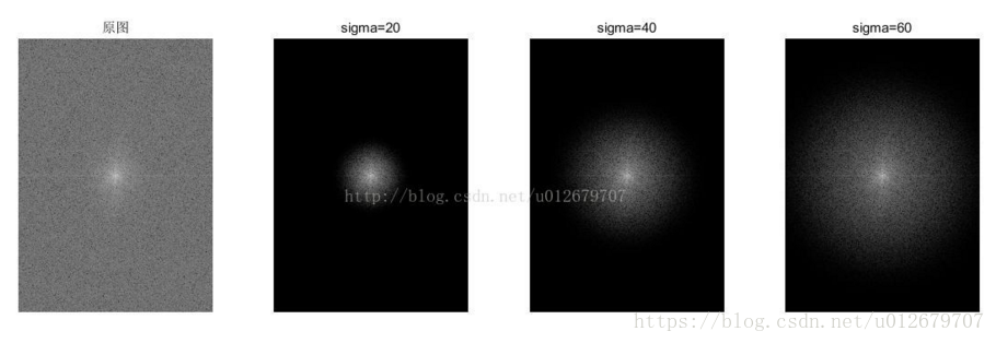
Compared with low-pass filter, Gaussian filter can effectively suppress noise and reduce the degree of image blur

cankao

Frequency domain high pass filter

Image sharpening can be achieved by attenuating low-frequency signals in the frequency domain

%Gaussian high pass filter imgaussfhpf.m
%{
Function: function ff=imgaussfhpf(I,sigma)
Function Description: construct Gaussian high pass filter
 Parameter Description: I: input image 
         sigma: standard deviation
 Return value: Gaussian high pass filter as large as the original image
 
%}
 
 
function ff=imgaussfhpf(I,sigma)
[M,N]=size(I);
 ff=ones(M,N);
 for i=1:M
     for j=1:N
         ff(i,j)= 1-exp( -((i-M/2)^2+(j-N/2)^2) /2/(sigma^2) ); %  1-(gauss)
        
     end
 end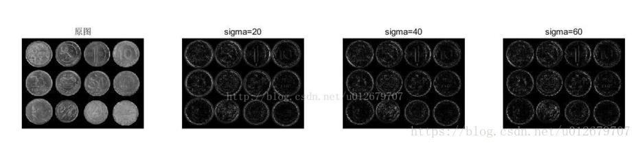

1. Gaussian high pass filter can extract edge information better;

2. The smaller the sigma is, the lower the cut-off frequency of Gauss high pass, the more low-frequency components pass through, the more inaccurate the edge extraction will contain more non edge information; (the requirements are too low and there are too many fishers in troubled waters) 3. The larger the sigma, the more accurate the edge extraction is, but it may contain incomplete edge information. (the requirements are too high and there is a fish in the net)

Laplacian filter

%laplace Filter filter imlapf.m
%{
Function: function ff=imlapf(I)
Function Description: Construction laplace Filter
 Parameter Description: I: input image 
       
Return value: the same size as the original image laplace Filter
 
%}
 
 
function ff=imlapf(I)
[M,N]=size(I);
 ff=ones(M,N);
 for i=1:M
     for j=1:N
         ff(i,j)= -((i-M/2)^2+(j-N/2)^2)  % 
        
     end
 end

Image processing evaluation index

Evaluation algorithm based on error sensitivity:

The simplest quality evaluation algorithms are mean square error (MSE) and peak signal - noise ratio (PSNR). MSE and PSNR are widely used in the field of image processing because of their low computational complexity and easy implementation. But the disadvantage is that there is no inevitable relationship between the values they give and the perceived quality of the image.

Peak signal-to-noise ratio PSNR

Evaluation of signal reconstruction quality in image compression and other fields

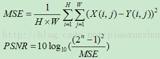
MSE is the mean square error of the current image X and the reference image Y, and H and W represent the height and width of the image respectively; n is the number of bits per pixel, generally 8, that is, the number of gray scales of pixels is 256. The unit of PSNR is dB. The larger the value, the smaller the distortion.

matlab code:

    function pnsr_result = psnr(img_ref,img_in)       
        %   img_ref is a high reference quality image   
        %   img_in is the denoise image    
        %   pnsr_result is the PSNR of the denoise image    
        width = size(img_ref,2);    
        heigh = size(img_ref,1);    
        if( width ~= size(img_in,2) || heigh ~= size(img_in,1) )    
            disp('Please check whether the input image and reference image have same size');    
            return    
        end    
        [a,b]=size(img_ref);      
        XX=double(img_ref) - double(img_in);      
        mse_value = sum(sum( XX.^2 ))/(a*b);      
        pnsr_result = 10*log10( 255*255 / mse_value );   
    end

SSIM

Signal to noise ratio (SNR)

SNR is the ratio of useful signal to noise signal

snr=10*log_{10}\frac{sigma(I2)}{sigma(I2-I1)}

function snr=SNR2(I,In)
% Calculate noise ratio
% I :original signal
% In:noisy signal
% snr=10*log10(sigma2(I2)/sigma2(I2-I1))
 
[~,~,nchannel]=size(I);
snr=0;
I=double(I);
In=double(In);
if nchannel==1
    Ps=sum(sum((I-mean(mean(I))).^2));%signal power
    Pn=sum(sum((I-In).^2));%noise power
    snr=10*log10(Ps/Pn);
elseif nchannel==3
    for i=1:3
        Ps=sum(sum((I(:,:,i)-mean(mean(I(:,:,i)))).^2));%signal power
        Pn=sum(sum((I(:,:,i)-In(:,:,i)).^2));%noise power
        snr=snr+10*log10(Ps/Pn);
    end
    snr=snr/3;
end

Evaluation algorithm based on structural similarity

other

Handling of overexposure

Calculate the inverse (255 image) of the current image, and then take the smaller of the current image and the inverse image as the value of the current pixel position.

min(image,(255-image))

Plus Masaic algorithm

Principle: use the center pixel to represent the neighborhood pixel Opencv Code:

uchar getPixel( IplImage* img, int row, int col, int k)
{
    return ((uchar*)img->imageData + row* img->widthStep)[col*img->nChannels +k];
}
 
void setPixel( IplImage* img, int row, int col, int k, uchar val)
{
    ((uchar*)img->imageData + row* img->widthStep)[col*img->nChannels +k] = val;
}

--

// nSize: size, odd
// Replace the value of the neighborhood with the value of the center pixel
void Masic(IplImage* img, IplImage* dst, int nSize)
{
    int offset = (nSize-1)/2;
    for ( int row = offset; row <img->height - offset; row= row+offset)
    {
        for( int col= offset; col<img->width - offset; col = col+offset)
        {
            int val0 = getPixel(img, row, col, 0);
            int val1 = getPixel(img, row, col, 1);
            int val2 = getPixel(img, row, col, 2);
            for ( int m= -offset; m<offset; m++)
            {
                for ( int n=-offset; n<offset; n++)
                {
                    setPixel(dst, row+m, col+n, 0, val0);
                    setPixel(dst, row+m, col+n, 1, val1);
                    setPixel(dst, row+m, col+n, 2, val2);
                }
            }
        }
    }
}