I. Frequency Domain Processing of Images

1.1 Concept of Frequency Domain Image Processing

Image processing in frequency domain is to transform the image into frequency domain, and then process the image in frequency domain. Its characteristic is fast operation.

The first step of frequency domain processing is to transform the image from time domain to frequency domain. Therefore, various transformations are the basis of image processing research.

1.2 Discrete Fourier Transform (DFT)

Fourier transform is discrete in both time domain and frequency domain. The sampling of time domain signal is transformed into sampling in discrete time Fourier transform frequency domain.

1.3 Fourier Transform Image Processing Example-Opencv

1.3.1 Principal Function

#include <opencv2/core/core.hpp>
#include <opencv2/highgui/highgui.hpp>
#include <opencv2/imgproc/imgproc.hpp>
#include <iostream>

using namespace std;
using namespace cv;

// Function declaration
void ImgDFT(Mat& inputImag_1, Mat&outputImg);

int main()
{
	double dx = 1.5, dy = 1.5; // Scaling factor

    // Load the image and display it
    Mat originImage_boy = imread("baby.png", 1);
    imshow("original_boy", originImage_boy);

     if (originImage_boy.empty()) {
     	return -1;
     }


    // Create renderings
    Mat resultImage;
    // resultImage.create(round(originImage_boy.rows), round(originImage_boy.cols), originImage_boy.type());

    // Recording time
    double timeClock = static_cast<double>(getTickCount());

    // function call
    // Different functions can be defined and invoked
    ImgDFT(originImage_boy, resultImage);
    

    // Output time
    timeClock = ((double)getTickCount() - timeClock) / getTickCount();
    cout << "run time:" << timeClock << "seconds" << endl;

    //  imshow("result",resultImage);
    waitKey(0);
    return 0;
}

Discrete Fourier Transform Function of 1.3.1 Image

// Function definition
// Computing images using dynamic addresses
void ImgDFT(Mat& inputImag_1, Mat& outputImg) {
	Mat srcGray;
	cvtColor(inputImag_1, srcGray, CV_RGB2GRAY); 

	int m = getOptimalDFTSize(srcGray.rows);
	int n = getOptimalDFTSize(srcGray.cols);

	Mat padded;

	//[1] The gray scale image is expanded to the optimum size, and the image is expanded to the right and the bottom, and the expanded boundary is filled with 0.
	copyMakeBorder(srcGray, padded, 0, m - srcGray.rows,0, n - srcGray.cols, BORDER_CONSTANT, Scalar::all(0));
	cout<<padded.size()<<endl;
	//[2] Allocate storage space for Fourier transform results.
	//Here we get two Mat s, one for storing dft transform and the other for storing imaginary part. Initially, the real part is the image itself, and the imaginary part is all zero.
	Mat planes[] = {Mat_<float>(padded), Mat::zeros(padded.size(),CV_32F)};
	Mat complexImg;
	//Integrating several single-channel mats into a multi-channel mat, where the fused complexImg has both real and imaginary parts
	merge(planes,2,complexImg);
 	// [3] Discrete Fourier Transform
	//Fourier transform is applied to the mat synthesized above to support in-situ operation. The result of Fourier transform is complex. Channel 1 contains real part and channel 2 contains imaginary part.
	dft(complexImg,complexImg);
	//The transformed result is divided into two mat s, one real part and one imaginary part, which is convenient for subsequent operation.
	// [4] Complex to Amplitude Conversion
	split(complexImg,planes); 
	// [5] scaling
	//This part is to calculate the amplitude of the dft transform. The range of the amplitude of the Fourier transform is too large to be displayed on the screen. High values are shown as white dots on the screen, while low values are black dots. The changes of high and low values can not be effectively distinguished. In order to highlight the continuity of high and low changes on the screen, we can replace the linear scale with logarithmic scale in order to display the magnitude. The calculation formula is as follows:
	//=> log(1 + sqrt(Re(DFT(I))^2 +Im(DFT(I))^2))
	magnitude(planes[0],planes[1],planes[0]);
	Mat mag = planes[0];
	mag += Scalar::all(1);
	log(mag, mag);
 	// [6] Shear and redistribution amplitude image limits
	//crop the spectrum, if it has an odd number of rows or columns
	//Pruning the spectrum, if the row or column of the image is odd, then the spectrum is asymmetric. Pruning is necessary.
	mag = mag(Rect(0, 0, mag.cols & -2, mag.rows & -2));
	Mat _magI = mag.clone();
	//The purpose of this step is still to display, but the magnitude is still beyond the display range [0,1]. We use normalize() function to normalize the magnitude to the display range.
	normalize(_magI, _magI, 0, 1, CV_MINMAX);
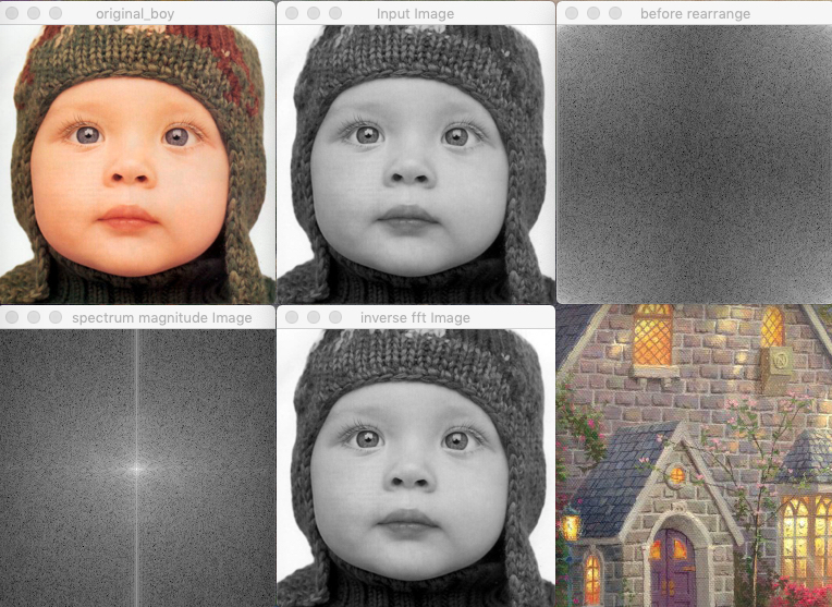
	imshow("before rearrange", _magI);
 
	//rearrange the quadrants of Fourier image
	//so that the origin is at the image center
	// [7] The quadrant is reassigned to move (0,0) to the image center.
	//In Digital Image Processing, the source image is centralized by multiplying (-1)^ (x+y) before Fourier transform.   
	//This is the centralization of Fourier transform results.
	int cx = mag.cols/2;
	int cy = mag.rows/2;
 
	Mat tmp;
	Mat q0(mag, Rect(0, 0, cx, cy));   //Top-Left - Create a ROI per quadrant
	Mat q1(mag, Rect(cx, 0, cx, cy));  //Top-Right
	Mat q2(mag, Rect(0, cy, cx, cy));  //Bottom-Left
	Mat q3(mag, Rect(cx, cy, cx, cy)); //Bottom-Right
 
	//swap quadrants(Top-Left with Bottom-Right)
	q0.copyTo(tmp);
	q3.copyTo(q0);
	tmp.copyTo(q3);
 
	// swap quadrant (Top-Rightwith Bottom-Left)
	q1.copyTo(tmp);
	q2.copyTo(q1);
	tmp.copyTo(q2);
 
	// [8] Normalization, using floating-point values between 0 and 1 to transform the matrix into a visual image format
	normalize(mag,mag, 0, 1, NORM_MINMAX);
	imshow("Input Image", srcGray);
	imshow("spectrum magnitude Image",mag);
 
	//Inverse Fourier Transform
	Mat ifft;
	idft(complexImg,ifft,DFT_REAL_OUTPUT);
	normalize(ifft,ifft,0,1,CV_MINMAX);
	imshow("inverse fft Image",ifft);

}

1.3.3 Image Fourier Transform Result Diagram