abstract
This report is based on MNIST handwritten numeral data set collected by National Institute of standards and technology. In the current era, there are still a large number of handwritten digits to deal with. Their recognition and classification is the key to solve the problem. In this paper, I practiced and experienced the classification of handwritten data in MNIST dataset. The main contents of this paper include: the record of the experimental process, the brief analysis of the experimental results, and the introduction of relevant methods. The experimental process is implemented by Python, using AutoEncoder dimension reduction method and MLP and FCN classification methods. The final conclusion is obtained by comparing the accuracy of the two classification methods.
Keywords: handwritten numeral recognition; Ultra high dimensional data; data classification
ABSTRACT
This report is based on MNIST handwritten digital data set collected by National Institute of Standards and Technology, NIST. In the current era, there are still a large number of handwritten digits to be processed, and their recognition and classification is the key to solve the problem. In this paper, I practice and experience the classification of handwritten data in MNIST data set. The main contents of this paper include: the recording of the experimental process, the brief analysis of the experimental results, and the introduction of the relevant methods. The experimental process is implemented by Python 3. The AutoEncoder, Multilayer Perceptron and Fully Convolutional Networks are used. The final conclusion is obtained by comparing the accuracy of the two classification methods.
Key words: Handwritten digit recognition, Ultra-high dimensional data, Data Classification
1 research background and significance
1.1 research background
1.1.1 origin
The National Institute of standards and technology has the need to recognize handwritten digits, so it collects and counts the handwritten digit styles from more than 200 people, arranges their handwriting images into MNIST data sets, and realizes the recognition of handwritten digits with algorithms; At the same time, MNIST data set also helps researchers evaluate and understand machine learning algorithms.
1.1.2 development
In 1998, LeCun realized handwritten numeral recognition based on MNIST data set with CNN algorithm in his paper "graduate based learning applied to document recognition".
MNIST has gradually become a well-known handwritten digital data set, which is widely used by more and more people. Related projects have become a classic example to be learned.
1.2 research significance
Experience MNIST data set and practice the use of relevant methods; Handwritten numeral recognition based on MNIST data set is realized in Python, and a better method is further determined according to the experimental results.
2 data sources
2.1 MNIST dataset
2.1.1 data set introduction
MNIST data set is a large handwritten numeral data set compiled by the National Institute of standards and technology of the United States, including 60000 training sets and 10000 test sets. The digital image has been processed, and each image file has a unified size of 28 * 28 pixels, including one of the numbers 0-9; The handwritten digits in the image are displayed in the center, which is convenient for operation and processing.
2.1.2 dataset official website
The official website of MNIST is: http://yann.lecun.com/exdb/mnist/index.html , from which the required data can be obtained.
3 empirical analysis
3.1 data preprocessing and dimensionality reduction
3.1.1 preparation
Unzip the downloaded mnist.zip file, including 1 npz file and 4 gz files. gz file stores vectors and multi-dimensional matrices, including handwritten digital images and labels; The npz file plays a role of integration. When writing Python code later, you can only read the npz file to obtain the content that needs to be used in the dataset.
import tensorflow
import keras
import matplotlib.pyplot as plt
import numpy as np

#The files involved in the original data have been uploaded to jupyter notebook
#Open npz file
mnist = np.load('mnist.npz')
tensorlow is a deep learning framework commonly used in the field of machine learning. It can be used to build neural network distributed learning and interactive system. It has the characteristics of strong universality and portability. It shows good results in applications such as handwriting recognition and image classification.
keras is an artificial neural network library, which can be used for various operations of deep learning model. It is installed and imported based on tensorflow in Python.
When using tensorflow and keras for the first time in Python 3, you need to use the pip install method for installation. It has been installed in advance here, so it is omitted.
3.1.2 set training set and test set
#Set train and test
x_train = mnist['x_train']
y_train = mnist['y_train']
x_test = mnist['x_test']
y_test = mnist['y_test']
In the process of machine learning, it is necessary to divide the data into training set and test set, train the model with the data of training set, and verify the effect of the model in the test set.
The mnist data set has been pre segmented, and only the training set and test set in the x and y directions need to be set respectively. You can also preview the set training set and test set.
3.1.3 preview data
#Preview an image
plt.figure(figsize=(5,5))
plt.imshow(x_train[300])
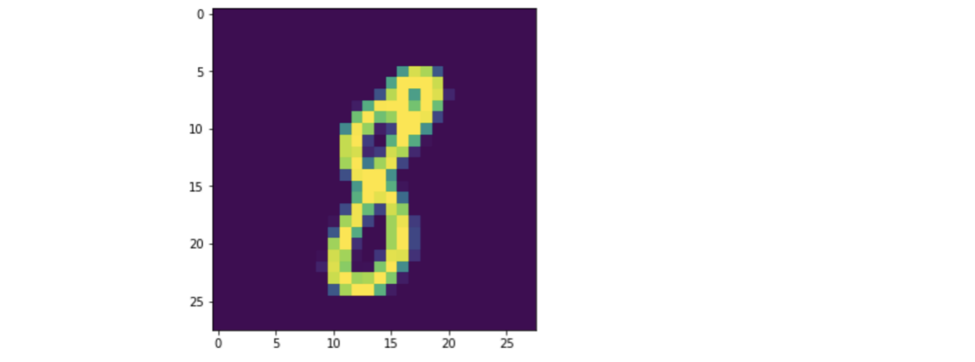
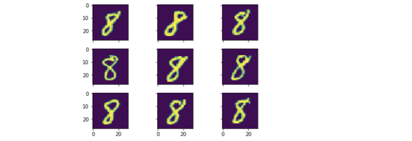
Before performing subsequent operations, the original handwritten digital image in mnist data is previewed to facilitate the understanding of the data set. Here, two preview methods are used to view a single number 8 in the data and multiple numbers 8 at the same time. According to the characteristics of mnist data set, each image contains different handwriting.
#You can also preview multiple images at once. We can see these handwritten numbers, each of which looks different
fig, ax = plt.subplots(
    nrows=3,
    ncols=3,
    sharex=True,
    sharey=True, )
ax = ax.flatten()
for i in range(9):
    img = x_train[y_train == 8][i]
    ax[i].imshow(img,interpolation='nearest')
plt.tight_layout()
plt.show()
3.1.4 viewing shapes
Use shape to view the size of each dimension of training set and test set respectively. The training set contains 60000 images, and the test set contains 10000 images, each in the form of 28 * 28 pixels.
3.1.5 normalization
Normalize the image data to simplify the calculation. Here, we need to convert the original [0255] to [0,1], and divide the training set and test set directly.
#Normalize image data
#Originally [0255], converted to [0,1]
x_train = x_train / 255
x_test = x_test / 255
3.1.6 Vectorization
In the above 3.1.4, it is determined that the image in the data is 28 * 28 pixels. For the normal execution of subsequent operations, each image needs to be converted into a vector with dimension 784.
#It is known from the above that each image is 28x28, and all of them are converted into 784 vectors
x_train = x_train.reshape(60000, 784)
x_test = x_test.reshape(10000, 784)
After conversion: becomes a vector, not an image

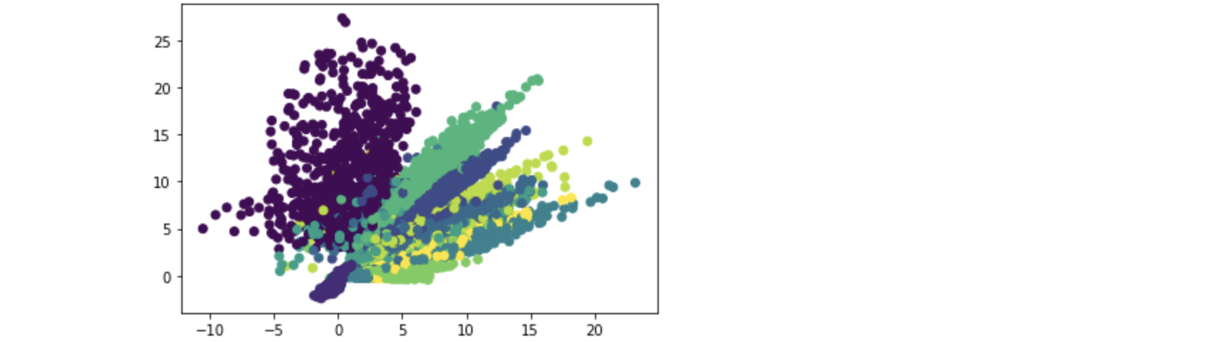
3.1.7 dimension reduction
Dimension reduction using AutoEncoder. The mechanism of AutoEncoder has been understood in 2.3. In order to obtain better visualization effect, epochs is set to 50 to reduce the data to two dimensions.
#Dimensionality reduction
x_train = x_train.reshape(x_train.shape[0], -1)
x_test = x_test.reshape(x_test.shape[0], -1)
encoding_dim = 2

encoder = keras.models.Sequential([
    keras.layers.Dense(128, activation='relu'),
    keras.layers.Dense(32, activation='relu'),
    keras.layers.Dense(8, activation='relu'),
    keras.layers.Dense(encoding_dim)])

decoder = keras.models.Sequential([
    keras.layers.Dense(8, activation='relu'),
    keras.layers.Dense(32, activation='relu'),
    keras.layers.Dense(128, activation='relu'),
    keras.layers.Dense(784, activation='tanh')])

AutoEncoder = keras.models.Sequential([encoder,decoder])
AutoEncoder.compile(optimizer='adam', loss='mse')
AutoEncoder.fit(x_train, x_train, epochs=50, batch_size=256)

predict = encoder.predict(x_test)
Output the reduced dimension image.
plt.scatter(predict[:, 0], predict[:, 1], c=y_test)
plt.show()
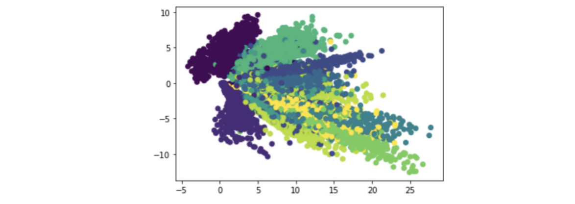
In addition, if AutoEncoder dimensionality reduction is performed again, the image will change. For example:
3.2 using MLP classification
3.2.1 building models
Here we want to use MLP multi-layer perceptron to classify MNIST data sets.
Among them, Sequential is the Sequential model in keras, which has linear structure order. Activation, density and dropout are common network layers of keras. The effect of activation is to assign an activation function to a layer; Density is a fully connected layer, which can be connected to the upper layer to obtain nonlinear combination; Dropout acts on the input data and will randomly disconnect part of the input to prevent over fitting.
from keras.models import Sequential
from keras.layers import Activation,Dense,Dropout
Use the above components to build a classification model including Softmax functions.
model = Sequential()
model.add(Dense(512, input_shape=(784,)))
model.add(Activation('relu'))
model.add(Dropout(0.2))
model.add(Dense(512))
model.add(Activation('relu'))
model.add(Dropout(0.2))
model.add(Dense(10))
model.add(Activation('softmax'))
3.2.2 training model
Apply the training set to the built model. After several attempts, it is found that the computer performance is limited, the number of iterations should not be too many, and the accuracy is not affected. Therefore, epochs is temporarily set to 10.
model.compile(optimizer='adam',loss='categorical_crossentropy', metrics=['accuracy'])

model.fit(x_train, y_train,
          batch_size=16, epochs=25,verbose=0,
          validation_data=(x_test, y_test))
3.2.3 evaluation model
Apply the test set to the model and calculate the accuracy. When epochs=10, the accuracy is 98.33%.
score = model.evaluate(x_test, y_test, verbose=0)
print('The accuracy is:', score[1])
You can also modify the number of iterations in 3.2.2 to increase epochs to 25 and test again.
It is found that the accuracy has little difference compared with that when epochs=10, or even decreases. It is speculated that this is because the number of iterations is not enough and the accuracy fluctuates to a certain extent.
3.3 using FCN classification
3.3.1 building models
Here, FCN is used to classify MNIST data sets. First, build the model. In order to distinguish it from the MLP method above, the relevant variables are named model2 and score2 during FCN construction. When constructing the FCN model, we should also use the Sequential model of keras and the common network layers such as Dense and Activation.
In terms of code, the biggest difference between FCN and MLP is that the Activation function used in the Activation layer of MLP is relu, while the Activation layer of FCN uses tanh.
The process of building FCN model is as follows:
model2 = Sequential()
model2.add(Dense(784, input_dim=784, kernel_initializer='normal',
                 activation= 'tanh'))
model2.add(Dense(512, kernel_initializer='normal',
                 activation= 'tanh'))
model2.add(Dense(512, kernel_initializer='normal',
                 activation= 'tanh'))
model2.add(Dense(10, kernel_initializer='normal',
                 activation= 'softmax'))
3.2.2 training model
After applying the training set, it is found that the iteration speed is much faster than that of MLP method. Therefore, epochs is taken as a larger 100 here, hoping to achieve higher accuracy.
model2.compile(optimizer='adam', loss='categorical_crossentropy', metrics=['accuracy'])

model2.fit(x_train, y_train, epochs=100, batch_size=200, verbose=1,
            validation_data=(x_test,y_test))
3.2.3 evaluation model
Applying the test set, the accuracy is 98.35%, which is considerable in value.
score2 = model2.evaluate(x_test,y_test, verbose=0)
print('The accuracy is:',score2[1])
4 Conclusion
In this paper, MNIST data set is used for experiment, and python 3 is used to write code in the whole process. In the preprocessing part, normalization and other means are used to reduce the dimension of data compression by using AutoEncoder. In addition, MLP and FCN are used to classify the data.
During the experiment, the accuracy of MLP and FCN was observed. The former was 98.19%, and the latter was 98.35%. FCN was slightly higher in value.
However, this comparison is problematic because the two methods are iterated for different times in the experiment.
Therefore, an experiment with epochs of 100 is added to control the variables as much as possible.
#MLP
model = Sequential()
model.add(Dense(512, input_shape=(784,)))
model.add(Activation('relu'))
model.add(Dropout(0.2))
model.add(Dense(512))
model.add(Activation('relu'))
model.add(Dropout(0.2))
model.add(Dense(10))
model.add(Activation('softmax'))
model.compile(optimizer='adam',loss='categorical_crossentropy', metrics=['accuracy'])
model.fit(x_train, y_train,
          batch_size=16, epochs=100,verbose=0,
          validation_data=(x_test, y_test))
score = model.evaluate(x_test, y_test, verbose=0)
print('MLP The accuracy of supplementary experiment is:', score[1])
#FCN
model2 = Sequential()
model2.add(Dense(784, input_dim=784, kernel_initializer='normal',
                 activation= 'tanh'))
model2.add(Dense(512, kernel_initializer='normal',
                 activation= 'tanh'))
model2.add(Dense(512, kernel_initializer='normal',
                 activation= 'tanh'))
model2.add(Dense(10, kernel_initializer='normal',
                 activation= 'softmax'))
model2.compile(optimizer='adam', loss='categorical_crossentropy', metrics=['accuracy'])
model2.fit(x_train, y_train, epochs=100, batch_size=200, verbose=1,
            validation_data=(x_test,y_test))
score2 = model2.evaluate(x_test,y_test, verbose=0)
print('FCN The accuracy of supplementary experiment is:',score2[1])
The results showed that the accuracy of MLP supplementary experiment was 98.53%, and that of FCN supplementary experiment was 98.34%.
Therefore, the classification accuracy of MLP method is higher than that of FCN method.