OpenCV for feature matching

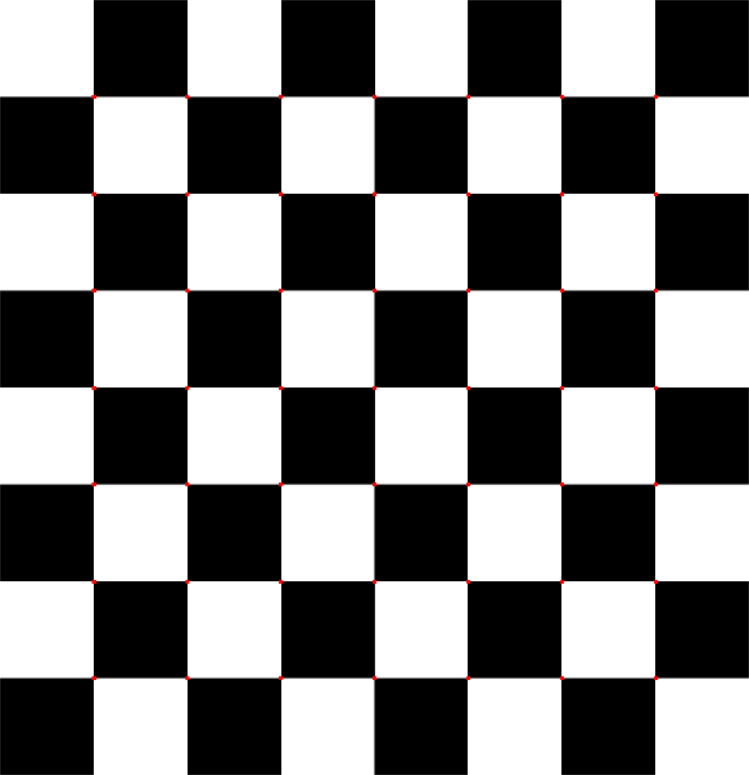
1.cornerHarris() for corner detection

Function CV2 in Open. CornerHarris() can be used for corner detection. The parameters are as follows:
* img - Input image with float32 data type.
blockSize - The size of the area to be considered in corner detection.
* ksize - window size used in Sobel derivation
* k - Harris corner detection equation for free parameters, the value parameter is [0,04,0.06].

import numpy as np
import cv2 as cv

filename = './image/chessboard.png'
img = cv.imread(filename)
x, y = img.shape[0:2]

gray = cv.cvtColor(img, cv.COLOR_BGR2GRAY)
gray = np.float32(gray)

dst = cv.cornerHarris(gray, 2, 3, 0.04)
a1 = dst > 0.01 * dst.max()
count1 = 0
for i in range(a1.shape[0]):
    for j in range(a1.shape[1]):
        if a1[i][j]:
            count1 += 1

print("Position of corner before expansion", count1)
# The function expands the input image with a specific structure element that determines the shape of the neighborhood during the expanding operation and replaces each point's pixel value with the maximum value on the corresponding neighborhood:
kernel = np.ones((16, 16))
dst = cv.dilate(dst, kernel)
# Mark the points found
a2 = dst > 0.01 * dst.max()
count2 = 0
for i in range(a2.shape[0]):
    for j in range(a2.shape[1]):
        if a2[i][j]:
            count2 += 1

print("Position of corner after expansion", count2)
print("Ratio before to after expansion", count2 / count1)


img[dst > 0.01 * dst.max()] = [0, 0, 255]
img_scale = cv.resize(img, (int(y / 6), int(x / 6)))
cv.imshow('dst', img_scale)

if cv.waitKey(0) & 0xff == 27:
    cv.destroyAllWindows()

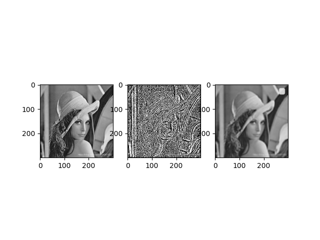
2. Laplacian Sharpening Picture

from PIL import Image
import numpy as np
from matplotlib import pyplot as plt

# Read in the original image
img = Image.open('./image/lenna.jpg')

# To reduce the calculated dimension, convert the image to grayscale
img_gray = img.convert('L')

# Get the pixel matrix of the converted grayscale
img_arr = np.array(img_gray)
h = img_arr.shape[0]  # That's ok
w = img_arr.shape[1]  # column

# Laplacian sharpens images using second-order differential
new_img_arr = np.zeros((h, w))  # Laplacian sharpened image pixel matrix
for i in range(2, h - 1):
    for j in range(2, w - 1):
        new_img_arr[i][j] = img_arr[i + 1, j] + img_arr[i - 1, j] + img_arr[i, j + 1] + img_arr[i, j - 1] - 4 * img_arr[
            i, j]

# Add the sharpened Laplacian image to the original image
laplace_img_arr = np.zeros((h, w))  # Pixel matrix from the addition of Laplacian sharpened and original images
for i in range(0, h):
    for j in range(0, w):
        laplace_img_arr[i][j] = new_img_arr[i][j] + img_arr[i][j]

img_laplace = Image.fromarray(np.uint8(new_img_arr))
img_laplace2 = Image.fromarray(np.uint8(laplace_img_arr))

plt.subplot(131), plt.imshow(img_gray, "gray")
plt.subplot(132), plt.imshow(img_laplace, "gray")
plt.subplot(133), plt.imshow(img_laplace2, "gray")
plt.legend()
plt.show()

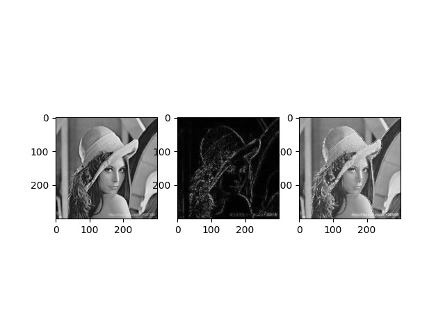
(2)OpenCV operator laplace sharpening
Function CV2 in Open. Laplacian() can be used for sharpening. The parameters are as follows
src - original image
ddepth - The depth of the image, -1 means the same depth as the original image. The depth of the target image must be greater than or equal to the depth of the original image
[Optional parameters]
dst - Target Image
The ksize-operator must be 1, 3, 5, 7 in size. Default 1
Scale - is the scale constant of the scaling derivative, with no scaling factor by default
delta - is an optional increment that will be added to the final dst, again, no additional values will be added to the DST by default
borderType - is the pattern used to determine the boundary of an image. The default value for this parameter is cv2.BORDER_DEFAULT.

import cv2 as cv
from matplotlib import pyplot as plt

img = cv.imread("./image/lenna.jpg", 0)

gray_lap = cv.Laplacian(img, cv.CV_16S, ksize=1)
dst = cv.convertScaleAbs(gray_lap)

img2 = dst + img
plt.subplot(131), plt.imshow(img, "gray")
plt.subplot(132), plt.imshow(dst, "gray")
plt.subplot(133), plt.imshow(img2, "gray")
plt.show()

3. SIFT determines the feature descriptor

1.sift = cv2.xfeatures2d.SIFT_create() instantiation

Parameter description: sift is an instantiated sift function

2.kp = sift.detect(gray, None) to find the key points in the image

Parameter description: kp represents the generated key point, gray represents the input grayscale.

3. ret = cv2.drawKeypoints(gray, kp, img) draw key points in the graph

Parameter description: gray for input picture, kp for key point, img for output picture

4.kp, dst = sift.compute(kp) calculates the SIFT eigenvectors corresponding to the critical points

Parameter description: kp represents the key point of input, dst represents the sift eigenvector of output, usually 128-dimensional

import numpy as np
import cv2 as cv

img = cv.imread('./image/home.jpg')
gray = cv.cvtColor(img, cv.COLOR_BGR2GRAY)

sift = cv.xfeatures2d.SIFT_create()
kp = sift.detect(gray, None)
img = cv.drawKeypoints(gray, kp, img)
kp, dst = sift.compute(gray, kp)

cv.imshow("SIFT", img)
cv.imwrite('./image/sift_keypoints.jpg', img)
cv.waitKey(0)
cv.destroyAllWindows()

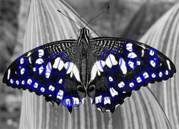
4.Surf identifies characteristics

import numpy as np
import cv2 as cv

img = cv.imread('./image/butterfly.jpg', 0)

# Create a SURF object. You can specify parameters here or later.
# Set here the threshold value of the Heisen matrix to 400
surf = cv.xfeatures2d.SURF_create(400)
# We set it to 50000. Remember, it is only used to represent pictures.
# In practice, it is best to set the value to 300-500
surf.setHessianThreshold(40000)
# Calculate key points and check their number.
kp, des = surf.detectAndCompute(img, None)
# Calculating the number of feature descriptors can be adjusted by adjusting the Heisen matrix threshold
print(len(kp))

img2 = cv.drawKeypoints(img, kp, None, (255, 0, 0), 4)

cv.imshow('surf', img2)

cv.waitKey(0)
cv.destroyAllWindows()

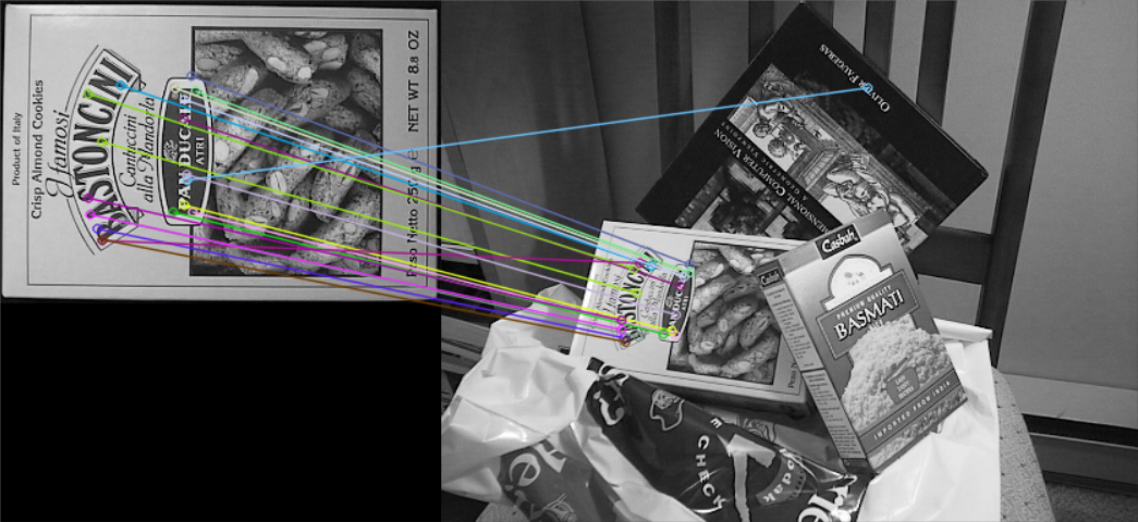
5.ORB identifies characteristics

import numpy as np
import cv2 as cv
import matplotlib.pyplot as plt

img1 = cv.imread('./image/box.png', 0)  # queryImage
img2 = cv.imread('./image/box_in_scene.png', 0)  # trainImage
# Initialize ORB
orb = cv.ORB_create()

# Identify key points on two graphs
kp1, des1 = orb.detectAndCompute(img1, None)
kp2, des2 = orb.detectAndCompute(img2, None)

# create BFMatcher object, BF is used to match feature points
bf = cv.BFMatcher(cv.NORM_HAMMING, crossCheck=True)
# Match descriptors.
matches = bf.match(des1, des2)
# Sort them in the order of their distance.
matches = sorted(matches, key=lambda x: x.distance)
# Draw first 10 matches.
img3 = cv.drawMatches(img1, kp1, img2, kp2, matches[:20], None, flags=2)
cv.imshow('ORB', img3)

cv.waitKey(0)
cv.destroyAllWindows()

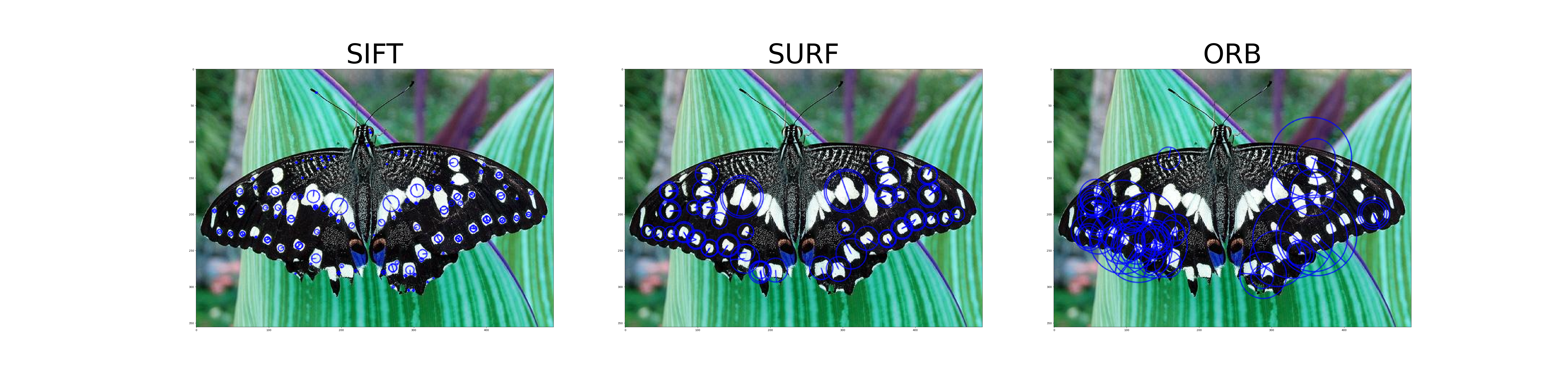
6. Compare SIFT SURF ORB

import cv2 as cv
from matplotlib import pyplot as plt
import numpy as np

img = cv.imread("./image/butterfly.jpg")
img_gray = cv.cvtColor(img, cv.COLOR_BGR2GRAY)

# Setting up three feature extraction processing objects
SIFT = cv.xfeatures2d.SIFT_create(200)
SURF = cv.xfeatures2d.SURF_create(40000)
ORB = cv.ORB_create(50)

# Determining key points and feature descriptors
kp_SIFT, des_SIFT = SIFT.detectAndCompute(img_gray, None)
kp_SURF, des_SURF = SURF.detectAndCompute(img_gray, None)
kp_ORB, des_ORB = ORB.detectAndCompute(img_gray, None)
print("SIFT Find feature points:{}；SURF Find feature points:{}，ORB Find feature points:{}".format(len(kp_SIFT), len(kp_SURF), len(kp_ORB)))

# Draw Feature Descriptor
plt.figure(figsize=(80, 20), dpi=100)
img_SIFT = cv.drawKeypoints(img, kp_SIFT, None, [0, 0, 255], 4)
img_SURF = cv.drawKeypoints(img, kp_SURF, None, [0, 0, 255], 4)
img_ORB = cv.drawKeypoints(img, kp_ORB, None, [0, 0, 255], 4)

# Draw Image
P1 = plt.subplot(131)
P1.set_title('SIFT', size=100), plt.imshow(img_SIFT)
P2 = plt.subplot(132)
P2.set_title('SURF', size=100), plt.imshow(img_SURF)
P3 = plt.subplot(133)
P3.set_title('ORB', size=100), plt.imshow(img_ORB)

plt.show()

Before Further Study

1. Traditional image segmentation methods

Image segmentation refers to dividing an image into several non-overlapping areas according to the characteristics of gray scale, color, texture and shape, and making these features show similarity in the same area, while showing obvious differences between different areas. Classical digital image segmentation algorithms are generally based on one of the two basic characteristics of gray values: discontinuity and similarity.

1.1 Threshold-based segmentation

Setting a certain gray threshold T can divide the image into two parts: the group of pixels larger than T and the group of pixels smaller than T. An appropriate threshold can accurately divide the image.

1.2 Edge-based segmentation method

The basic idea of image segmentation method based on edge detection is to determine the edge pixels in the image first, and then connect them together to form the desired area boundary.
There are five operators:
1. roberts operator

2. prewitt Operator

3. sobel operator

4. LoG Operator (Second Order Differential Operator)
1. The image is convoluted with a Gaussian filter, which smoothes the image and reduces the noise. Isolated noise points and small structures are filtered out.
_2. In edge detection, only those points with the maximum local gradient are considered as edge points. Laplace operator is used to convert edge points to zero intersections, and zero intersections are used to detect edges.
_3. The disadvantage is that the original edges are smoothed to some extent while filtering the noise.

5. canny Operators
_The basic idea of Canny operator method for detecting edge points is to find the local maximum value of image gradient.
Following these three criteria, the design and implementation steps of Canny operator are as follows:
(1) First convolute the image with a Gaussian filter template to smooth the image;
(2) Calculate the magnitude and direction of the gradient using the differential operator;
(3) nonmaximal suppression of the gradient amplitude. That is, traversing an image, if the gray value of a pixel is not the largest compared with the gray value of two pixels in the gradient direction, then the pixel value is set to 0, that is, not the edge;
(4) Use the double threshold algorithm to detect and connect edges. Even if two thresholds are calculated using the cumulative histogram, any higher threshold value must be an edge. Whatever is less than the low threshold must not be an edge. If the detection result is larger than the low threshold but smaller than the high threshold, it depends on whether there are edge pixels in the adjacent pixels of this pixel that exceed the high threshold. If there are, the pixel is the edge, otherwise it is not the edge.
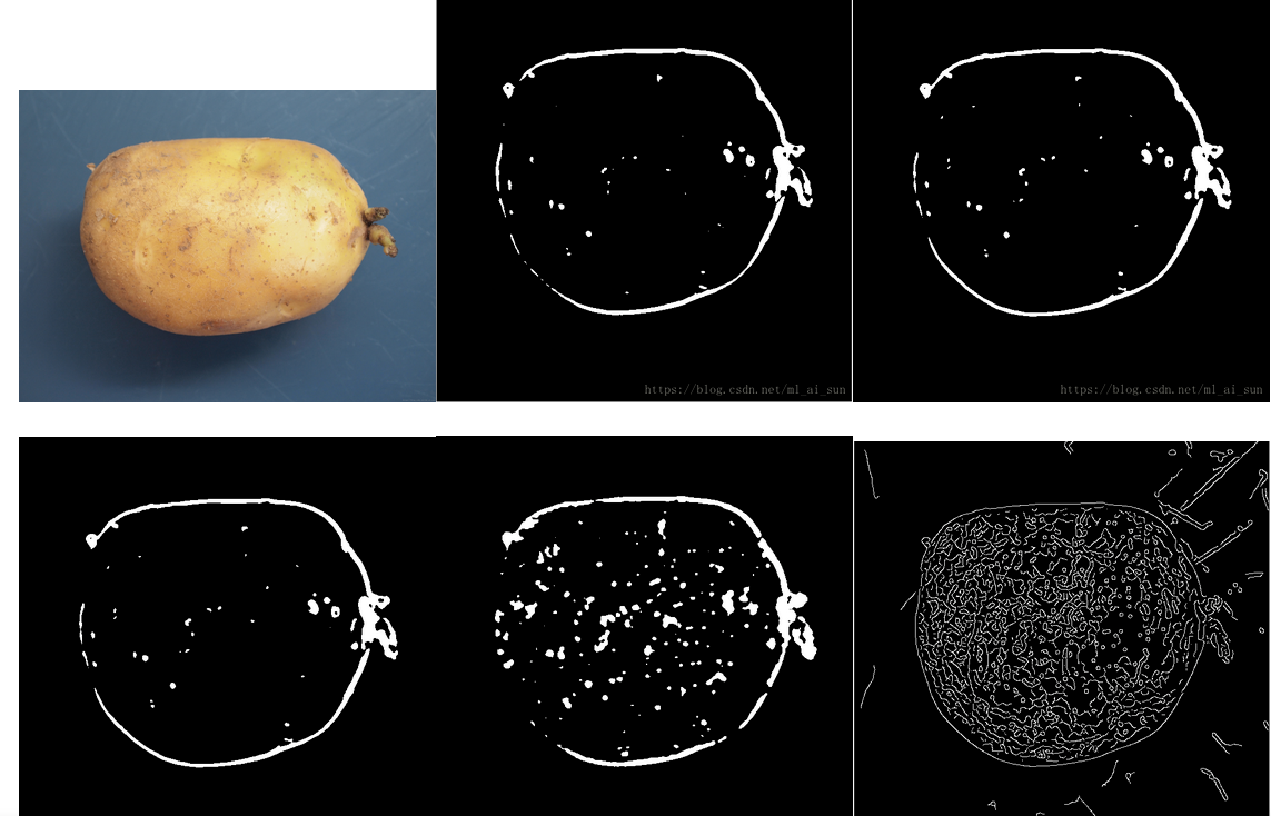From left to right are original, roberts, prewitt, sobel, LoG, canny

Edge detection is more suitable for images with low noise, not suitable for complex images, second-order differential operator is very sensitive to noise

1.3 Region-based segmentation method

This method divides the image into different regions according to the similarity criterion, mainly including seed region growth method, region split merge method and watershed method.

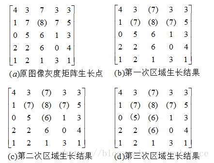
1.3.1 Zonal Growth Method

Figure (a) is the original image, and the numbers represent the gray scale of the pixels. The initial growth point is a pixel with a gray value of 8, which is denoted as f(i,j). Within 8 neighborhoods, the growth criterion is that the difference between the grey value of the point to be measured and the grey value of the growing point is 1 or 0. Figure (b) is then merged because after the first region growth, f(i-1,j)=7, f(i,j-1)=7, f(i,j+1)=7, and the gray value of the growing point differs by 1. chart © f(i+1,j)=6 is merged after the second growth. Fig. (d) After the third growth, f(i+1,j-1)=5, f(i+2,j)=6 are merged, so there are no pixel points satisfying the growth criteria and the growth stops.

1.3.2 watershed algorithm

The color image is grayed, then the gradient map is calculated. Finally, a watershed algorithm is applied on the basis of the gradient map to get the edge line of the segment image.

The entire process of the watershed algorithm:

1. Classify all the pixels in the gradient image according to their gray values and set a geodesic distance threshold.
2. Find the pixel point with the smallest gray value (the default is marked as the lowest gray value, or you can mark it yourself) and let the threshold grow from the minimum value, which is the starting point.
3. As the horizontal plane grows, it encounters surrounding neighboring pixels, measures the geodesic distance from these pixels to the starting point (the lowest point of gray value), and submerges them if it is less than the set threshold. Otherwise, dams are set on these pixels, and these neighboring pixels are classified.
4. As the horizontal plane gets higher, more and higher dams will be set up until the maximum of the grayscale value, all areas will meet on the watershed line, and these dams will partition the entire image pixels.

Watershed algorithm needs to consider over-segmentation

1.4 Graph-based segmentation methods

1.4.1Graph Cuts Split

Graph cuts is a very useful and popular energy optimization algorithm that is widely used in computer vision for ** Image segmentation, stereo vision, Image matting, etc.

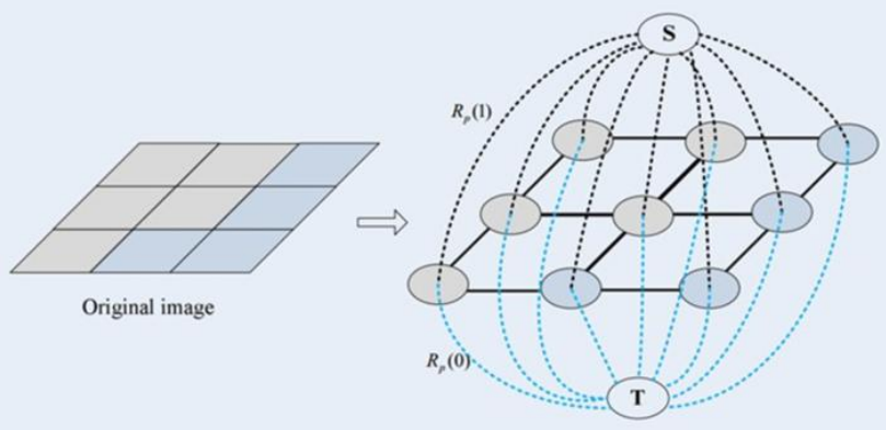
(1) First establish two vertices
The first common vertex corresponds to each pixel in the image. The connection of each two neighborhood vertices (corresponding to each two neighborhood pixels in the image) is an edge.
The other two terminal vertices are S (source: foreground) and T (sink: background). Each normal vertex is connected to these two terminal vertices to form the second edge (the foreground and background points are artificially selected,)

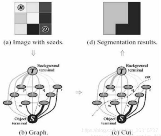
(2) To obtain a cut
Cuts in Graph Cuts refers to a collection of edges in which disconnection of all edges results in the separation of the residual S and T graphs and is therefore called secant.

(3) Find the smallest cut
If a cut has the smallest sum of ownership values of its edges, then this is called the smallest cut, which divides the vertices of a graph into two disjoint subsets, S and T, where s < S, T < T and S T=V. These two subsets correspond to the foreground and background pixel sets of the image, which is equivalent to the completion of image segmentation.

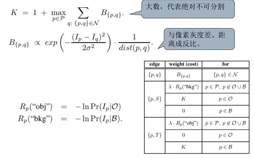
What is the method for calculating weights?

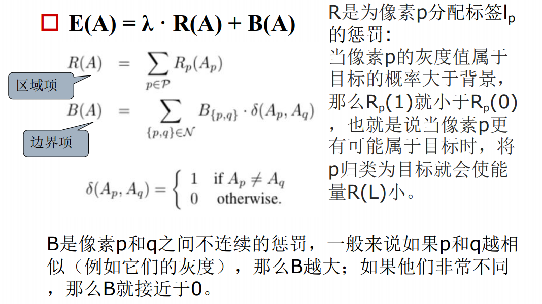
Where R(A) is the region term, B(A) is the boundary term, and λ They are important factors between the region and boundary terms that determine how much they affect energy. In colloquial terms: the dashed line between the terminal vertex and each pixel point is R(A), the solid line between each pixel point is B(A), and the coefficient λ Is a weight factor that determines which factor has a greater influence.
If λ 0, then only the boundary factor is considered, not the regional factor. E(A) represents the weight, which is the loss function, also known as the energy function. The goal of the graph cut is to optimize the energy function to minimize its value.

1.4.2 GrabCut Split

Grab is equivalent to an optimized version of Graph CUT:
The Graph cut algorithm calculates the probability of foreground and background based on the proportion of the histogram of the gray value in the pixel point (lp) gray value in the foreground and background [which foreground and background need to be marked beforehand, you need to tell Graph in advance which background is which?Which is foreground]
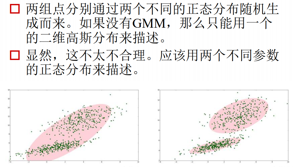
However, Grab cut is calculated based on the Gaussian Mixture Model (GMM), which calculates the probability of foreground and background clustering in each iteration.

The steps are as follows:
1. Enter a rectangle. All areas outside the rectangle must be backgrounds. What's inside the rectangle is unknown. Similarly, any action the user takes to determine the foreground and background will not be changed by the program.
2. The computer will make an initialization mark for our input image. It marks the foreground and background pixels.
3. Use a Gaussian Mixture Model (GMM) to model foreground and background
4. Based on our input, GMM will learn and create new pixel distributions. Pixels with unknown classifications (either foreground or background) can be classified based on their pixel relationship to known classifications (background, for example).
5. This creates a picture based on the distribution of pixels. The nodes in the graph are pixel points. There are two nodes besides the pixel point being a node: Source_node and ink_ Node. All foreground pixels are in Source_ Nodes are connected. All background pixels and sink_ Nodes are connected.
6. Connect Pixels to Source_ Node/end_ The weight of nodes'edges is determined by the probability that they belong to the same class. The weight between two pixels is determined by the edge information or the similarity of the two pixels. If two pixels have very different colors, the edges between them will have very small weights.
7. Use the mincut algorithm to segment the above image. It divides the image into Source_based on the least-cost equation Node and ink_ Node. The cost equation is the sum of the weights of all the edges that have been trimmed. After clipping, all connections to Source_node pixels are considered foreground, all connected to Sink_ The pixels of the node are considered background.
8. Continue this process until the classification converges.

(2) What is GMM**
Similar to the concept of clustering, classifying based on the distribution of points
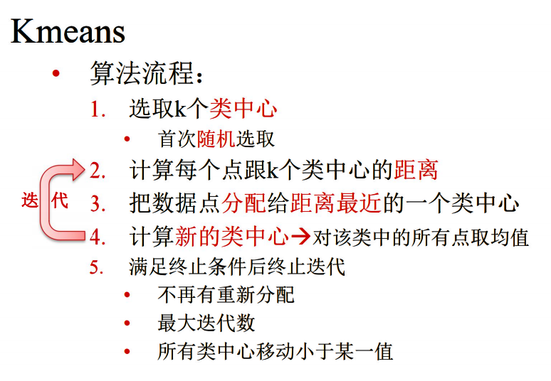
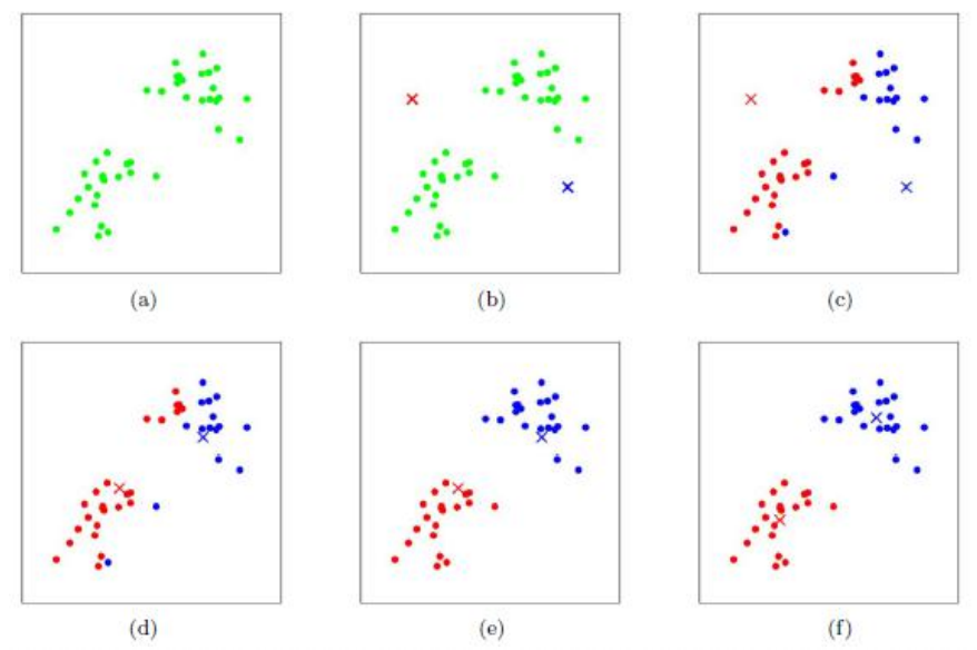
The iteration method to determine the GMM model is K-Means:
Number of cluster centers taken in K
The iteration process is to group the cluster centers belonging to the background in the foreground into the background. Only the future remains

(3) The nature of GrabCut:
- Iterate Graph Cuts
- Optimize color models for foreground and background
- Energy decreases with iteration
--The split results are getting better and better

2. Face detection

2.1 Haar cascade classifier

Haar classifier = Haar-like feature + integral graph method + AdaBoost + cascade;
A complete post about face detection using Haar cascade classifier

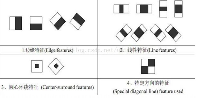
2.1.1 Haar-like Review

The feature template has two rectangles, white and black, and defines the feature values of the template as the pixels in the white rectangle and subtracts the sum of the pixels in the black rectangle. There are 15 templates:
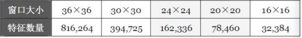
How many Haar-like features do you want to select?
There are many choices based on 15 templates and picture sizes, template sizes and locations:

2.1.2 Adaboost cascade classifier

Adaboost is a classifier based on cascade classification model. The following is an illustration of a cascade classification model:
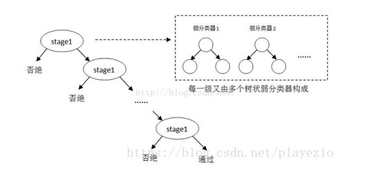Each of these stage s represents a first-level strong classifier. A positive sample is considered when the detection window passes through all the strong classifiers, otherwise it is rejected. In fact, not only is a strong classifier a tree structure, but every weak classifier in a strong classifier is also a tree structure. Because each strong classifier can discriminate negative samples very accurately, once negative target bits are detected, the following strong classifier is not called anymore, which reduces a lot of detection time. Because many of the areas to be detected in an image are negative samples, so complex detection of many negative samples is abandoned by the cascade classifier at the beginning of the classifier, so the speed of the cascade classifier is very fast. Only positive samples are sent to the next strong classifier for re-examination, which ensures that the possibility of false positive for the last positive output sample is very low.

How are cascade classifiers trained?
First, each weak classifier needs to be trained, then each weak classifier is combined according to a certain combination strategy to get a strong classifier, which is roughly as follows:
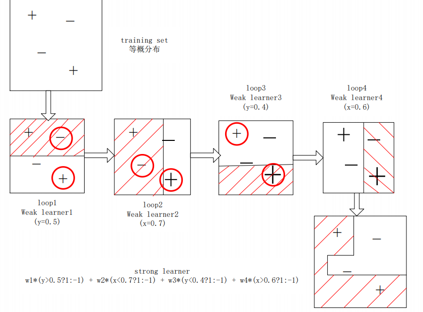Training a weak classifier means that under the current weight distribution, the weights of samples with bad estimation by the weak classifier increase continuously, and the optimal threshold of f is determined so that the classification error of all training samples by the weak classifier is the lowest.
Weak classifier is to select a feature from this huge number of features, which can distinguish face or non-face with the lowest error rate. The only requirement of a weak classifier is that it can distinguish face from non-face image with a slightly lower error rate than 50%.
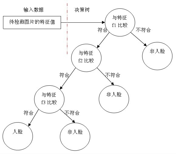A weak classifier is a decision tree similar to the one shown above. The basic weak classifier contains only one Haar-like feature.

We train several strong classifiers and then combine them in a cascade to get the Haar classifier that we ultimately want.

2.1.3 Face Recognition Steps

From the above, we can summarize the five steps of training the Haar classifier:

1. Prepare face and non-face sample sets;

2. Calculating eigenvalues and integral graphs;

3. Select T excellent eigenvalues (i.e. optimal weak classifier);

4. Pass this T optimal weak classifier to AdaBoost for training.

5. Cascade, that is, strong association of strong classifiers.

Before you start, it is important to remember that with the 20*20 window as an example, there are 78,460 features, and then T excellent features (i.e. the optimal weak classifier) are filtered out. This T optimal weak classifier is then passed to AdaBoost for training to get a strong classifier, and the strong classifier is cascaded.

2.2 HOG+SVM Pedestrian Detection (Target Detection)

A more detailed post to review

2.2.1 HOG implementation steps

(1) Image standardization (adjusting image contrast)
The main purpose is to reduce the influence of illumination factors, reduce the impact of local shadows and illumination changes on the image, and standardize (or normalize) the color space of the input image using Gamma correction method.

(2) Image smoothing
For gray-scale images, in order to remove noise, Gaussian function is used to smooth them first, but in some cases, it is better not to smooth them.

(3) Edge direction calculation
Calculates the gradient of each pixel of the image, including direction and size, with a special formula for amplitude and direction

(4) Histogram calculation

First, the image is divided into small cell units (cell units can be rectangular or circular), such as 8 × 8. Then the gradient histogram of each cell unit is counted to get a descriptor of the cell unit.
Then make up a block of several cell units, such as 2 × Two cell units form a block. By concatenating descriptors of each cell unit within a block, a block's HIG descriptor can be obtained.
Note: Typically, a 9-Bin histogram with a range of 180 degrees (one bin=20 degrees) is used.

(5) block normalization
Local contrast normalization is required for gradients because the absolute values of gradients vary widely due to changes in local illumination and the contrast of foreground and background. Normalization further compresses light, shadow, and edges so that the eigenvectors have changes in light, shadow, and edges Robustness.

(6) HOG feature extraction from samples
The final step is to extract HOG features from all the blocks in a sample and combine them into the final feature vector to feed into the classifier.
Calculate features with examples:
For example, for 128 × 64 input pictures (all image sizes I mentioned later refer to h × w), each block is made up of 2 × Two cells, each consisting of 8 × Eight pixel points, each cell extracts a 9-bin histogram with a cell size as a step. There are 15 scan windows in the horizontal direction and 7 scan windows in the vertical direction. That is, there are 15 7 2 9=3780 features.

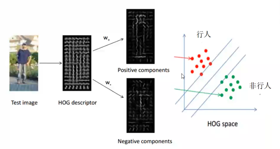
2.2.2 Distinguishing HOG characteristics between pedestrians and non-pedestrians using SVM

2.3 DPM

DPM can be seen as an extension of HOG (Histogrrams of Oriented Gradients), and the general idea is consistent with HOG. The gradient direction histogram is calculated, and then the gradient Model of the object is trained with SVM (Surpport Vector Machine). With such templates, you can use them directly for classification. A simple understanding is that the Model matches the target. DPM has only made a lot of improvements in the Model.

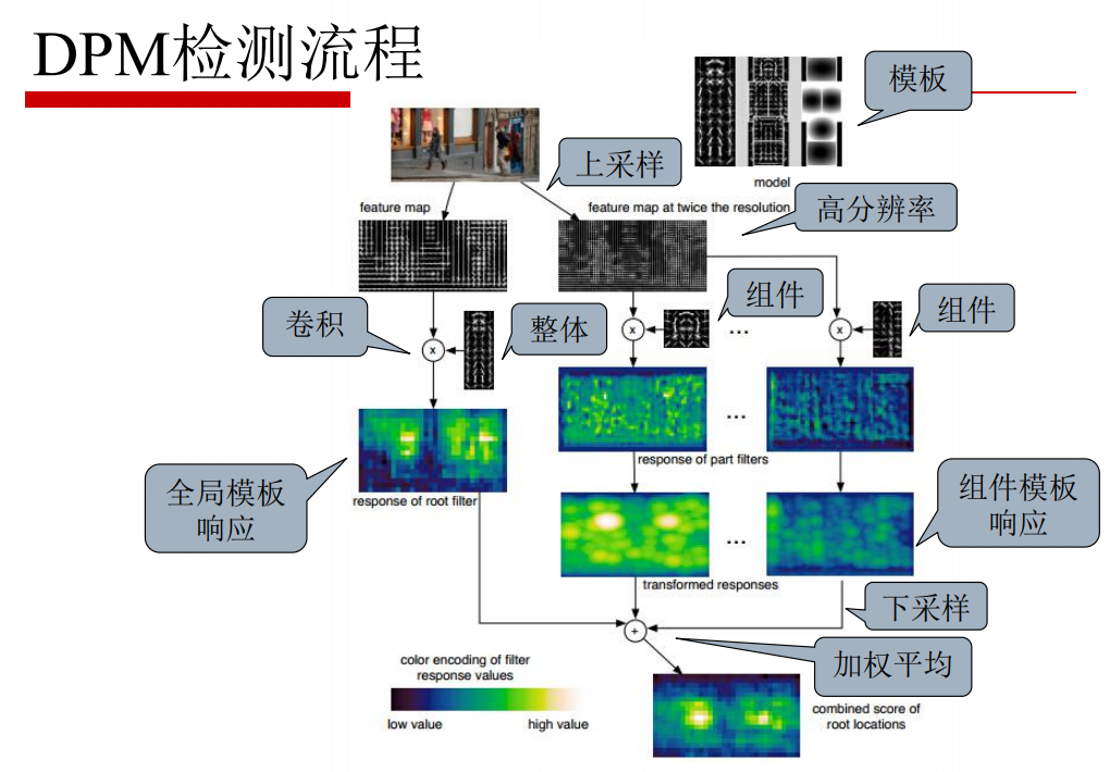
Detection process:
(1) For any input image, extract its DPM feature map, then sample the original image on a Gaussian pyramid, and extract its DPM feature map.
(2) Convolve the DPM feature map of the original image and the trained Root filter to get the response map of the Root filter.
(3) The DPM feature map of a 2-fold image is convoluted with the trained Part filter to get the response map of the Part filter.
(4) Then downsampling its fine Gauss pyramid so that the Root filter response map and the Artfilter response map have the same resolution.
(5) It is then weighted averaged to obtain the final response graph. Higher brightness means greater response value.

2.4 References:

Detailed Adaboost algorithm (haar face detection)

DPM(Deformable Parts Model) - Principle (1)

Detailed explanation of DPM (Deformable Part Model) principles

leetcode(111 112)

Minimum depth of leetcode111 binary tree

Recursively find the smallest, but remember that the end point of a cotyledon is that it has no cotyledons, not that it is currently empty.
Consider also the case where root==None

class Solution:
    def minDepth(self, root: TreeNode) -> int:
        if root is None:
            return 0
        if (not root.left) and (not root.right):
            return 1
        
        deepl=self.minDepth(root.left)
        deepr=self.minDepth(root.right)
        if deepr==0:
            deepr=100000
        if deepl==0:
            deepl=100000

        return min(deepl,deepr)+1

leetcode112 112. Path Sum

Recursive implementation, no difficulty

class Solution:
    def hasPathSum(self, root: Optional[TreeNode], targetSum: int) -> bool:
        if root is None:
            return False       
        if (not root.right) and (not root.left):
            if targetSum-root.val==0:
                return True
            else:
                return False
        
        targetSum-=root.val
        flagl=self.hasPathSum(root.left,targetSum)
        flagr=self.hasPathSum(root.right,targetSum)

        return (flagl)or(flagr)