1. Introduction
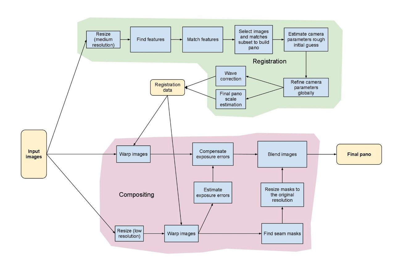
image mosaic is a direction of integrators in the field of traditional computer vision. The steps involved mainly include: feature point extraction, feature matching, image registration, image fusion, etc. Figure 1.1 below is the flow chart of opencv image stitching. There are many research directions involved in image stitching. For example, there are commonly used SIFT, SURF, ORB, etc. in the direction of feature extraction. These feature extraction methods are also widely used in the slam direction. Therefore, if you have spare efforts, it is very necessary to clarify these implementation details for establishing your own knowledge system.
2. opencv stitcher
opencv has a directly encapsulated Stitcher class, which basically calls an interface to complete all stitching steps and obtain stitched images. Test case picture reference resources.
2.1 example code
The following is an example code for calling the interface:
#include "opencv2/opencv.hpp"
#include "logging.hpp"
#include <string>

void stitchImg(const std::vector<cv::Mat>& imgs, cv::Mat& pano)
{
	//Set the splicing image warp mode, including PANORAMA and SCANS
	//panorama: the image will be projected onto a spherical or cylindrical surface for stitching
	//scans: by default, there is no illumination compensation and cylindrical projection, and it is spliced directly through affine transformation
    cv::Stitcher::Mode mode = cv::Stitcher::PANORAMA;
    cv::Ptr<cv::Stitcher> stitcher = cv::Stitcher::create(mode);
    cv::Stitcher::Status status = stitcher->stitch(imgs, pano);
    if(cv::Stitcher::OK != status){
        LOG(INFO) << "failed to stitch images, err code: " << (int)status;
    }
}

int main(int argc, char* argv[])
{
    std::string pic_path = "data/img/*";
    std::string pic_pattern = ".jpg";

    if(2 == argc){
        pic_path = std::string(argv[1]);
    }else if(3 == argc){
        pic_path = std::string(argv[1]);
        pic_pattern = std::string(argv[2]);
    }else{
        LOG(INFO) << "default value";
    }
    std::vector<cv::String> img_names;
    std::vector<cv::Mat> imgs;
    pic_pattern = pic_path + pic_pattern;
    cv::glob(pic_pattern, img_names);
    if(img_names.empty()){
        LOG(INFO) << "no images";
        return -1;
    }
    for(size_t i = 0; i < img_names.size(); ++i){
        cv::Mat img = cv::imread(img_names[i]);
        imgs.push_back(img.clone());
    }
    cv::Mat pano;
    stitchImg(imgs, pano);
    if(!pano.empty()){
        cv::imshow("pano", pano);
        cv::waitKey(0);
    }
    return 0;
}
2.2 example effect
-
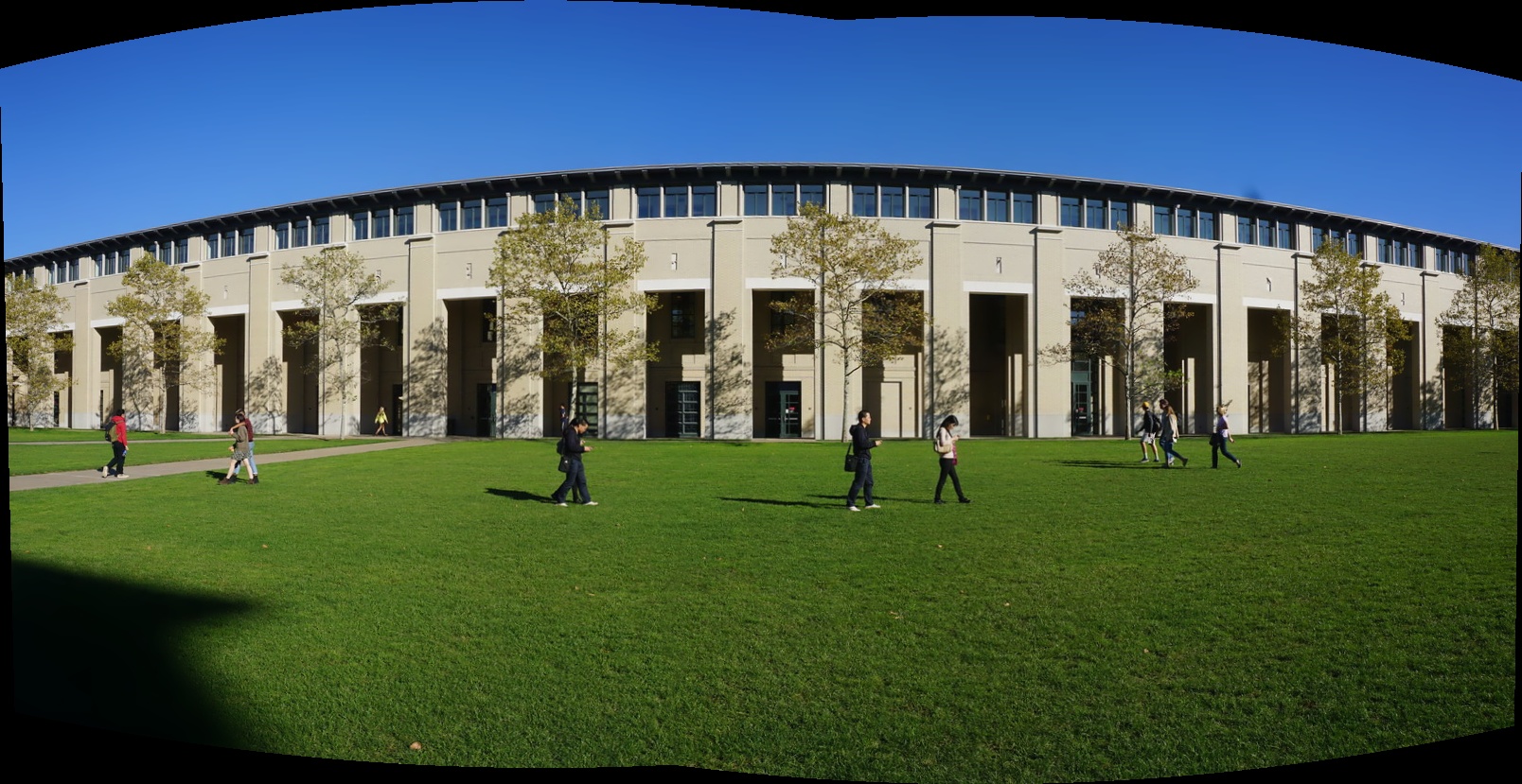
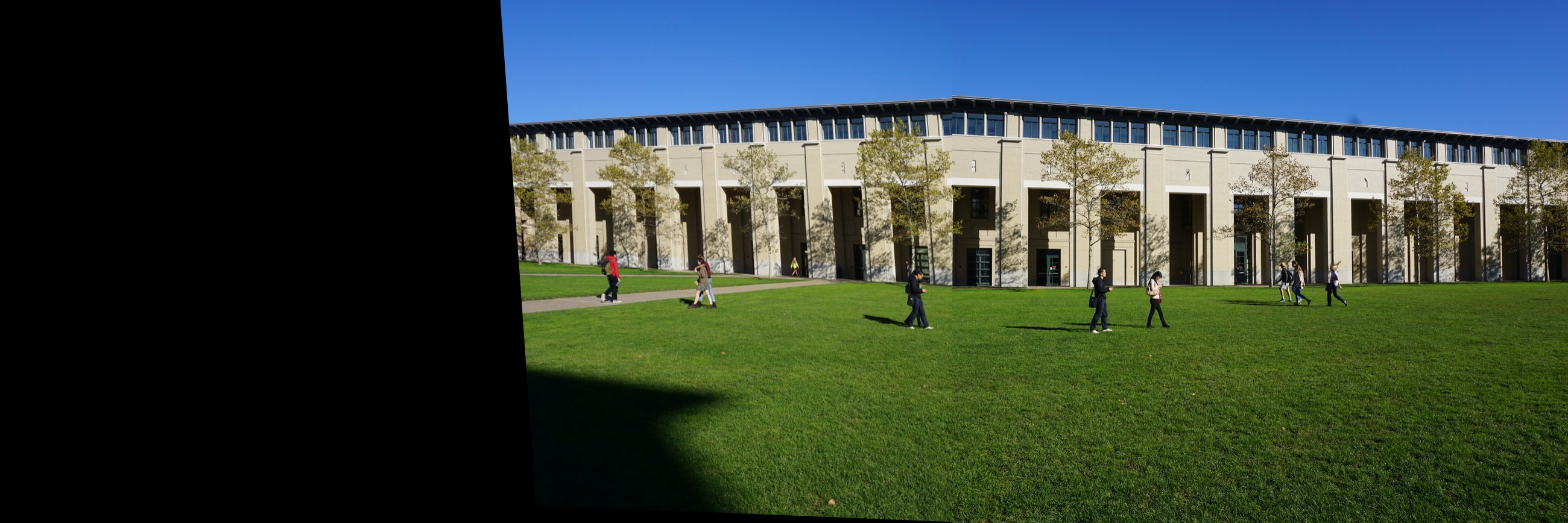
mode = panorama
CMU scene splicing 1
-
mode=scans
CMU scene splicing 2
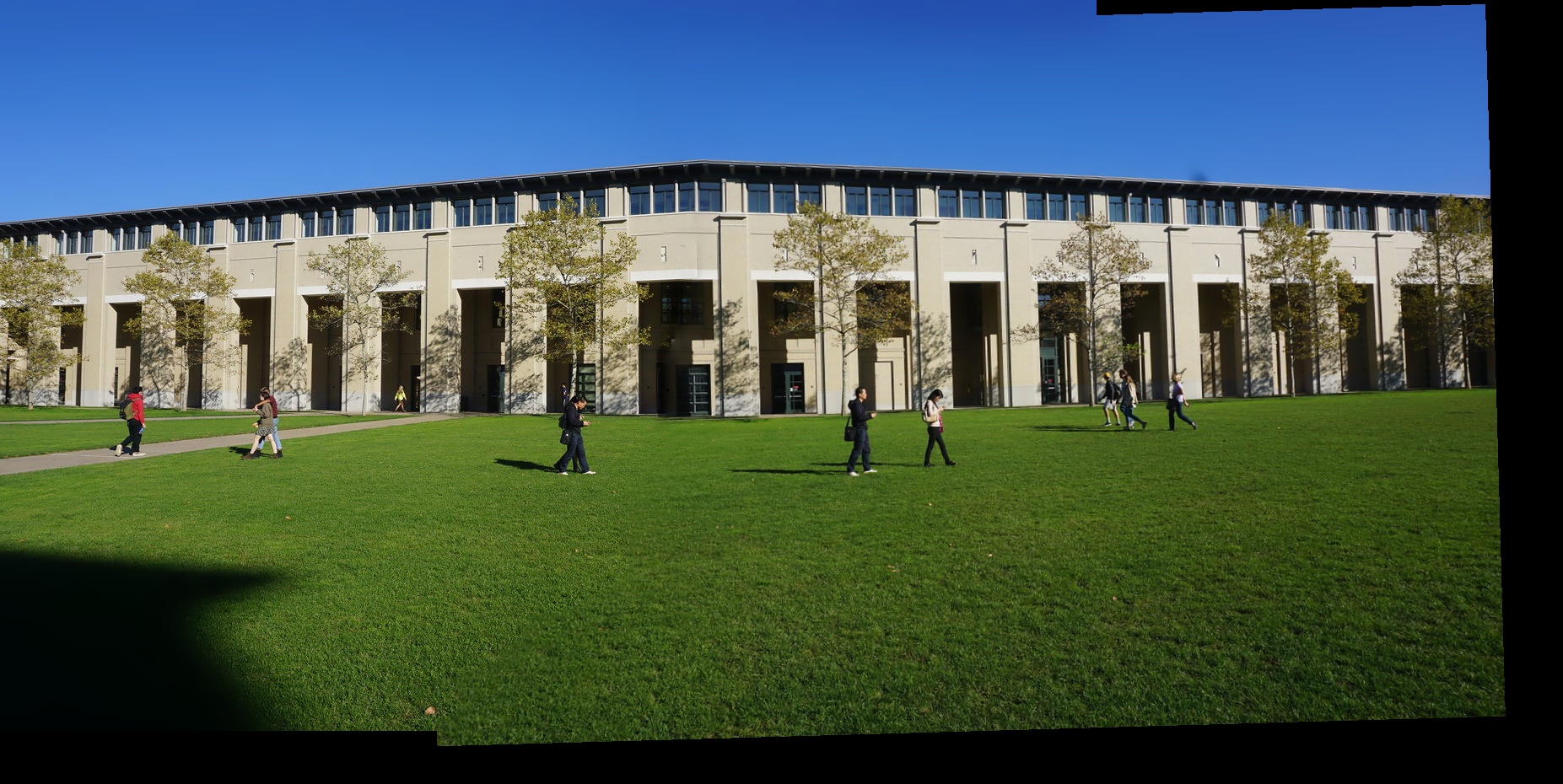
The above two groups of CMU scene comparison images illustrate the difference between PANORAMA and SCANS. The former will project the image on a cylindrical surface, and the PANORAMA will be curved, while SCANS only has affine transformation, so the mosaic images basically retain the straight-line parallel relationship of the original image.
3. Simplified splicing
in this section, we are going to dig some pits. When looking at the details of opencv stitcher, first simply imitate and realize the splicing of scans mode to see the effect of splicing. The basic idea is:
- First, set a canvas. The width is the sum of the widths of all images, and the height is the maximum height of all images. The default value is 0;
- Take the image on the right as the reference image, that is, transform the image on the left and then fuse it with the image on the right;
3.1 feature extraction
commonly used feature extraction mainly includes SIFT, SURF and ORB. ORB is fast and used more in other visual tasks, but the accuracy is not as high as the first two.
void featureExtract(const std::vector<cv::Mat> &imgs,
                    std::vector<std::vector<cv::KeyPoint>> &keyPoints,
                    std::vector<cv::Mat> &imageDescs)
{
    keyPoints.clear();
    imageDescs.clear();
    //Extracting feature points
    int minHessian       = 800;
    cv::Ptr<cv::ORB> orbDetector = cv::ORB::create(minHessian);
    for (int i = 0; i < imgs.size(); ++i) {
        std::vector<cv::KeyPoint> keyPoint;
        //Gray image conversion
        cv::Mat image;
        cvtColor(imgs[i], image, cv::COLOR_BGR2GRAY);
        orbDetector->detect(image, keyPoint);
        keyPoints.push_back(keyPoint);
        cv::Mat imageDesc1;
        orbDetector->compute(image, keyPoint, imageDesc1);
        /*imageDesc needs to be converted to floating-point type, otherwise an error will occur. Unsupported format or combination of formats in buildIndex using FLANN algorithm*/
        imageDesc1.convertTo(imageDesc1, CV_32F);
        imageDescs.push_back(imageDesc1.clone());
    }
}
3.2 feature matching
this step determines the pairing relationship of feature points between images according to the feature points of the image, so as to obtain the transformation matrix H. This h is the transformation of the whole image. Now, in order to solve some parallax problems, someone divides the grid on the image, and then calculates the transformation matrix H separately for each grid.
void featureMatching(const std::vector<cv::Mat> &imgs,
                     const std::vector<std::vector<cv::KeyPoint>> &keyPoints,
                     const std::vector<cv::Mat> &imageDescs,
                     std::vector<std::vector<cv::Point2f>> &optimalMatchePoint)
{
    optimalMatchePoint.clear();
    //The matching feature points are obtained and the optimal pairing is extracted. Here, the hypothesis is sequential input, and the hypothesis used in the test is two graphs
    cv::FlannBasedMatcher matcher;
    std::vector<cv::DMatch> matchePoints;
    matcher.match(imageDescs[0], imageDescs[1], matchePoints, cv::Mat());

    sort(matchePoints.begin(), matchePoints.end());//Feature point sorting
    //Obtain the top N optimal matching feature points
    std::vector<cv::Point2f> imagePoints1, imagePoints2;
    for (int i = 0; i < MAX_OPTIMAL_POINT_NUM; i++) {
        imagePoints1.push_back(keyPoints[0][matchePoints[i].queryIdx].pt);
        imagePoints2.push_back(keyPoints[1][matchePoints[i].trainIdx].pt);
    }
    optimalMatchePoint.push_back(std::vector<cv::Point2f>{imagePoints1[0], imagePoints1[3], imagePoints1[6]});
    optimalMatchePoint.push_back(std::vector<cv::Point2f>{imagePoints2[0], imagePoints2[3], imagePoints2[6]});
}
when using orb feature extraction, there are many mismatched points. The above three points match the correct points according to the display, which will be used to estimate the affine transformation matrix H. The internal processing of opencv uses RANSAC algorithm for estimation. I have omitted this step here.
3.3 estimating affine transformation matrix
the three strongest matching points are obtained in the previous step. In this step, H can be calculated directly. Before calculation, move the image on the right to the right of the canvas
void getAffineMat(std::vector<std::vector<cv::Point2f>>& optimalMatchePoint,
                  int left_cols, std::vector<cv::Mat>& Hs)
{
    std::vector<cv::Point2f> newMatchingPt;
    for (int i = 0; i < optimalMatchePoint[1].size(); i++) {
        cv::Point2f pt = optimalMatchePoint[1][i];
        pt.x += left_cols;
        newMatchingPt.push_back(pt);
    }
	//The transformation matrix of the image on the left, the feature points of the image on the right are moved, and the image on the left needs to be transformed to the feature point position of the image on the right on the canvas
    cv::Mat homo1 = getAffineTransform(optimalMatchePoint[0], newMatchingPt);
	//The transformation matrix of the right image, that is, the right image is moved to the right side of the canvas
    cv::Mat homo2 = getAffineTransform(optimalMatchePoint[1], newMatchingPt);

    Hs.push_back(homo1);
    Hs.push_back(homo2);
}
3.4 mosaic image
after determining the transformation matrix, take the feature point with the strongest response as the fusion center of the two images, and the left and right sides of the center correspond to two images respectively. This splicing processing method is very rough. For images taken only by translation, they can still be spliced together, but if rotation or wrong time center is added, the splicing dislocation is very serious. Another point is image fusion. Here, a dividing line is directly selected as the basis for selecting the pixels of the original image. If the transition is not smooth enough, there will be dislocation.
void getPano2(std::vector<cv::Mat> &imgs, const std::vector<cv::Mat> &H, cv::Point2f &optimalPt, cv::Mat &pano)
{
    //Taking the right image as a reference, the left image is changed to coincide with the right image through affine transformation, and the strongest response feature point is taken as the center of the fusion of the two images
    //The default panorama canvas size is: width = left width + right. width, height = std::max(left.height, right.height)
    int pano_width  = imgs[0].cols + imgs[1].cols;
    int pano_height = std::max(imgs[0].rows, imgs[1].rows);
    pano            = cv::Mat::zeros(cv::Size(pano_width, pano_height), CV_8UC3);
    cv::Mat img_trans0, img_trans1;
    img_trans0 = cv::Mat::zeros(pano.size(), CV_8UC3);
    img_trans1 = cv::Mat::zeros(pano.size(), CV_8UC3);
	//After affine change, the original image has been located at the corresponding position of the panorama
    cv::warpAffine(imgs[0], img_trans0, H[0], pano.size());
    cv::warpAffine(imgs[1], img_trans1, H[1], pano.size());

	//Strongest response characteristic point
    cv::Mat trans_pt = (cv::Mat_<double>(3, 1) << optimalPt.x, optimalPt.y, 1.0f);
	//The position of the most responsive feature point on the canvas
    trans_pt = H[0]*trans_pt;

	//Determine the area to be selected for the two images
    cv::Rect left_roi  = cv::Rect(0, 0, trans_pt.at<double>(0, 0), pano_height);
    cv::Rect right_roi = cv::Rect(trans_pt.at<double>(0, 0), 0,
            pano_width - trans_pt.at<double>(0, 0) + 1, pano_height);
	//Copy the selected area pixels to the canvas
    img_trans0(left_roi).copyTo(pano(left_roi));
    img_trans1(right_roi).copyTo(pano(right_roi));
    cv::imshow("pano", pano);
    cv::waitKey(0);
}

int main(int argc, char *argv[])
{
    cv::Mat image01 = cv::imread("data/img/medium11.jpg");
    cv::resize(image01, image01, cv::Size(image01.cols, image01.rows + 1));
    cv::Mat image02 = cv::imread("data/img/medium12.jpg");
    cv::resize(image02, image02, cv::Size(image02.cols, image02.rows + 1));
    std::vector<cv::Mat> imgs = {image01, image02};
    std::vector<std::vector<cv::KeyPoint>> keyPoints;
    std::vector<std::vector<cv::Point2f>> optimalMatchePoint;
    std::vector<cv::Mat> imageDescs;
    featureExtract(imgs, keyPoints, imageDescs);
    featureMatching(imgs, keyPoints, imageDescs, optimalMatchePoint);

    std::vector<cv::Point2f> newMatchingPt;
    for (int i = 0; i < optimalMatchePoint[1].size(); i++) {
        cv::Point2f pt = optimalMatchePoint[1][i];
        pt.x += imgs[0].cols;
        newMatchingPt.push_back(pt);
    }
    cv::Mat homo1 = getAffineTransform(optimalMatchePoint[0], newMatchingPt);
    cv::Mat homo2 = getAffineTransform(optimalMatchePoint[1], newMatchingPt);

    std::vector<cv::Mat> Hs = {homo1, homo2};
    cv::Mat pano;
    //getPano1(imgs, Hs, pano);
    getPano2(imgs, Hs, optimalMatchePoint[0][0], pano);
    return 0;
}
3.5 simplified splicing effect
- Image mosaic effect with only translation change
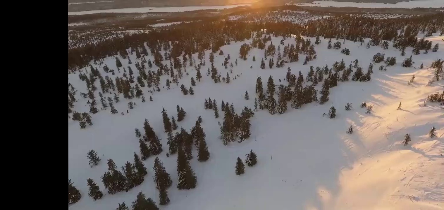
- Image mosaic with rotation change
it's not much effect. The dislocation can be clearly seen in Figure 3.5.2, and there is an obvious inclination on the left side of the whole splicing diagram. There are many reasons for dislocation. There is no good fusion transition algorithm, the rotation change of the camera is not taken into account, and the splicing seam position is not found well. If the picture is inclined and unnatural, it is caused by selecting a single picture as the reference picture and transforming other images to their coordinate system. Take these questions to see how opencv is implemented internally.
4. Opencv sticcher module
opencv provides stiching in the sample code_ detailed. CPP example, which contains the implementation steps of each module. We usually require real-time splicing in actual use, and we can't meet this requirement by directly adjusting the interface, especially at the arm embedded end, which requires us to find out the implementation details and find the optimization points. I'm only here for sticching_ detailed. Some details in CPP are of interest, so time-consuming statistics, scaling and selecting fusion areas are removed.
according to the opencv stitching flow chart in Figure 1.1, the main steps in opencv stitcher are:
- registration
- feature extraction
- Feature matching
- image registration
- Camera internal parameter estimation
- Waveform correction
- compositing
- Image transformation
- Illumination compensation
- Find seam
- Image fusion
registration is mainly used to obtain the matching relationship between images, estimate the internal and external parameters of the camera, and optimize the parameters using BA algorithm. The compositing part is to transform and fuse the image after obtaining the parameters, and use algorithms such as illumination compensation to improve the picture consistency. Later, we will also study in these two modules.