Introduction to LeNet neural network

LeNet neural network was proposed by Yan LeCun, one of the three giants of deep learning. He is also the father of convolutional neural networks (CNN). LeNet is mainly used for handwritten character recognition and classification, and has been used in American banks. The implementation of LeNet establishes the structure of CNN. Now many contents of neural network can be seen in the network structure of LeNet, such as convolution layer, Pooling layer and ReLU layer. Although LeNet was put forward as early as the 1990s, due to the lack of large-scale training data and the low performance of computer hardware, the effect of LeNet neural network in dealing with complex problems is not ideal. Although the structure of LeNet network is relatively simple, it is just suitable for the introduction of neural network.

LeNet neural network structure

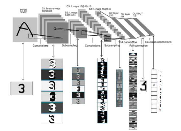
The neural network structure diagram of LeNet is as follows:

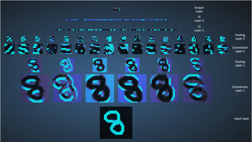
The execution flow chart of LeNet network is as follows:

Parameter changes of LeNet layers

• C1
  Input size: 32 * 32
  Core size: 5 * 5
  Number of cores: 6
  Output size: 28 * 28 * 6
  Number of training parameters: (5 * 5 + 1) * 6 = 156
  Number of connections: (5 * 5 + 1) * 6 * (32-2-2) * (32-2-2) = 122304

• S2
  Input size: 28 * 28 * 6
  Core size: 2 * 2
  Number of cores: 1
  Output size: 14 * 14 * 6
  Number of training parameters: 2 * 6 = 12, 2=(w,b)
  Number of connections: (2 * 2 + 1) * 1 * 14 * 14 * 6 = 5880

• C3
  Input size: 14 * 14 * 6
  Core size: 5 * 5
  Number of cores: 16
  Output size: 10 * 10 * 16
  Number of training parameters: 6 * (3 * 5 * 5 + 1) + 6 * (4 * 5 * 5 + 1) + 3 * (4 * 5 * 5 + 1) + 1 * (6 * 5 * 5 + 1) = 1516
  Number of connections: (6 * (3 * 5 * 5 + 1) + 6 * (4 * 5 * 5 + 1) + 3 * (4 * 5 * 5 + 1) + 1 * (6 * 5 * 5 + 1)) * 10 * 10 = 151600

• S4
  Input size: 10 * 10 * 16
  Core size: 2 * 2
  Number of cores: 1
  Output size: 5 * 5 * 16
  Number of training parameters: 2 * 16 = 32
  Number of connections: (2 * 2 + 1) * 1 * 5 * 5 * 16 = 2000

• C5
  Input size: 5 * 5 * 16
  Core size: 5 * 5
  Number of cores: 120
  Output size: 120 * 1 * 1
  Number of training parameters: (5 * 5 * 16 + 1) * 120 * 1 * 1 = 48120 (because it is fully connected)
  Number of connections: (5 * 5 * 16 + 1) * 120 * 1 * 1 = 48120

• F6
  Input size: 120
  Output size: 84
  Number of training parameters: (120 + 1) * 84 = 10164
  Number of connections: (120 + 1) * 84 = 10164

LeNet layer 3 (convolution operation)

It is noteworthy that the third layer of LeNet, LeNet layer 3 (layer C3) is also a convolution layer. The size of convolution cores is still 5 * 5, but the number of convolution cores becomes 16. The input of the third layer is 6 feature maps of 14 * 14, and the size of convolution cores is 5 * 5. Therefore, the size of feature map output after convolution is 10 * 10. Since there are 16 convolution cores, it is expected to output 16 feature maps, but since there are 6 feature maps input, it is necessary to adjust External treatment. The relationship between the input 6 feature maps and the output 16 feature maps is as follows:

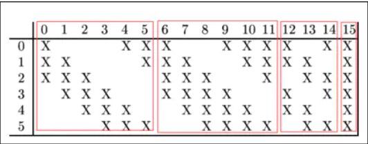
As shown in the figure above, the first convolution kernel processes the first three input feature maps to obtain a new feature map.

Letnet (pytoch version)

model.py

import torch.nn as nn
import torch.nn.functional as F

class LeNet(nn.Module):
    def __init__(self):
        super(LeNet,self).__init__()
        self.conv1 = nn.Conv2d(3,16,5)
        self.pool1 = nn.MaxPool2d(2,2)
        self.conv2 = nn.Conv2d(16,32,5)
        self.pool2 = nn.MaxPool2d(2,2)
        self.fc1 = nn.Linear(32*5*5,120)
        self.fc2 = nn.Linear(120,84)
        self.fc3 = nn.Linear(84,10)
    
    def forward(self, x):
        x = F.relu(self.conv1(x))#input(3,32,32) output(16,28,28)
        x = self.pool1(x) #output(16，14，14)
        x = F.relu(self.conv2(x)) #output(32,10.10)
        x = self.pool2(x) #output(32,5,5)
        x = x.view(-1,32*5*5) #output(5*5*32)
        x = F.relu(self.fc1(x)) #output(120)
        x = F.relu(self.fc2(x)) #output(84)
        x = self.fc3(x) #output(10)
        return x

#model debugging
import torch

#Define shape
input1 = torch.rand([32,3,32,32])
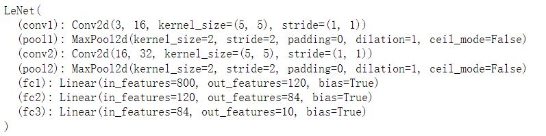
model = LeNet()#instantiation 
print(model)
#Input network
output = model(input1)

train.py

#train.py

import torch
import torchvision
import torch.nn as nn
import torch.optim as optim
import torchvision.transforms as transforms
from torchvision import transforms, datasets, utils
import matplotlib.pyplot as plt
import numpy as np


#device : GPU or CPU
device = torch.device("cuda:0" if torch.cuda.is_available() else "cpu")
print(device)


transform = transforms.Compose(
    [transforms.ToTensor(),
     transforms.Normalize((0.5, 0.5, 0.5), (0.5, 0.5, 0.5))])

# 50000 training pictures
train_set = torchvision.datasets.CIFAR10(root='./data', train=True,
                                         download=False, transform=transform)
train_loader = torch.utils.data.DataLoader(train_set, batch_size=36,
                                           shuffle=False, num_workers=0)

# 10000 verification pictures
val_set = torchvision.datasets.CIFAR10(root='./data', train=False,
                                       download=False, transform=transform)
val_loader = torch.utils.data.DataLoader(val_set, batch_size=5000,
                                         shuffle=False, num_workers=0)
val_data_iter = iter(val_loader)
val_image, val_label = val_data_iter.next()
print(val_image.size())
# print(train_set.class_to_idx)
# classes = ('plane', 'car', 'bird', 'cat',
#           'deer', 'dog', 'frog', 'horse', 'ship', 'truck')
#
#
# #Before displaying the image, you need to validate it_ Batch in loader_ Change size to 4
# aaa = train_set.class_to_idx
# cla_dict = dict((val, key) for key, val in aaa.items())
# def imshow(img):
#     img = img / 2 + 0.5  # unnormalize
#     npimg = img.numpy()
#     plt.imshow(np.transpose(npimg, (1, 2, 0)))
#     plt.show()
#
# print(' '.join('%5s' % cla_dict[val_label[j].item()] for j in range(4)))
# imshow(utils.make_grid(val_image))




net = LeNet()
net.to(device)

loss_function = nn.CrossEntropyLoss()
#Define optimizer
optimizer = optim.Adam(net.parameters(), lr=0.001)

#Training process
for epoch in range(10):  # loop over the dataset multiple times

    running_loss = 0.0 #Cumulative loss
    for step, data in enumerate(train_loader, start=0):
        # get the inputs; data is a list of [inputs, labels]
        inputs, labels = data
        #print(inputs.size(), labels.size())
        # zero the parameter gradients
        optimizer.zero_grad()#If the historical gradient is not cleared, the calculated historical gradient will be accumulated
        # forward + backward + optimize
        outputs = net(inputs.to(device))
        loss = loss_function(outputs, labels.to(device))
        loss.backward()
        optimizer.step()

        # print statistics
        running_loss += loss.item()
        if step % 500 == 499:    # print every 500 mini-batches
            with torch.no_grad():#Context manager
                outputs = net(val_image.to(device))  # [batch, 10]
                predict_y = torch.max(outputs, dim=1)[1]
                accuracy = (predict_y == val_label.to(device)).sum().item() / val_label.size(0)

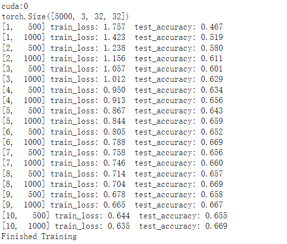
                print('[%d, %5d] train_loss: %.3f  test_accuracy: %.3f' %
                      (epoch + 1, step + 1, running_loss / 500, accuracy))
                running_loss = 0.0

print('Finished Training')

save_path = './Lenet.pth'
torch.save(net.state_dict(), save_path)