1. Preface
For the image with low original contrast, we can improve the contrast to enhance the recognition of the image, improve the visual effect of the image, convert it into a form more suitable for human and machine processing, remove useless information and improve the use value. Typical algorithms such as CT image enhancement, fog and rain removal, vein enhancement and so on.
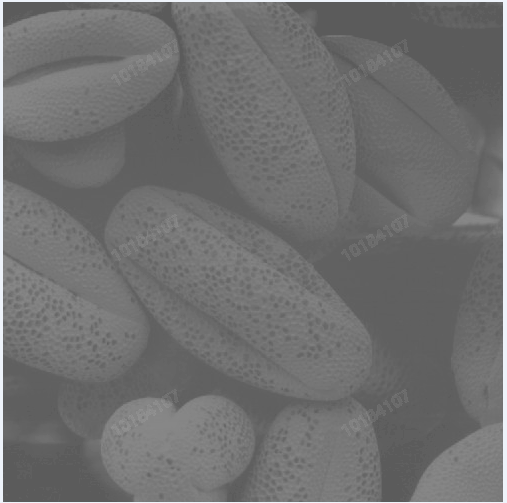
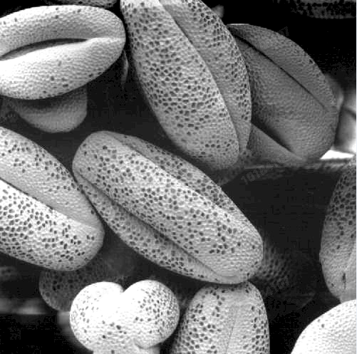
Considering the human visual characteristics, if the gray histogram of an image is evenly distributed, Then the image looks better (theoretically); of course, if further image classification or machine learning is needed, image preprocessing and enhancement is also helpful to target recognition and retrieval. As shown in the figure below, it is about image enhancement in the book digital image processing Matlab Edition (Gonzalez) (example of histogram equalization). It can be seen intuitively that the contrast of the left image is low and the image is hazy, which is very unnatural. The right image is very suitable for the visual characteristics of human eyes, and the contrast, recognition and even comfort have been greatly improved.
Then, in this chapter, we will mainly talk about the MATLAB & FPGA implementation of several basic image enhancement algorithms. Generally speaking, the commonly used image enhancement algorithms not only include contrast, histogram, noise reduction filtering, sharpness saturation and so on, but also belong to the image enhancement in the field of ISP. However, this chapter mainly focuses on histogram equalization and image enhancement of various contrast algorithms. Other contents will be further introduced in subsequent chapters.
2. Histogram equalization principle
Histogram equalization, also known as histogram stretching, is a simple and effective image enhancement technology. It changes the gray level of each pixel in the image by changing the histogram distribution of the image. It is mainly used to enhance the contrast of the image with small dynamic range. Because the gray distribution of the original image may be concentrated in a narrow range, As a result, the image is not clear enough (as shown on the left in the above figure), and insufficient exposure will concentrate the gray level of the image in the low brightness range. Histogram equalization can transform the histogram of the original image into a form of uniform distribution, which increases the dynamic range of gray value difference between pixels, so as to enhance the overall contrast of the image.
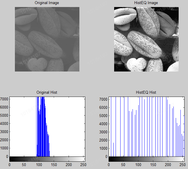
In other words, The basic principle of histogram equalization is to broaden the gray value with more pixels in the image (i.e. the gray value that plays a major role in the picture), and the gray value with less pixels (that is, the gray value that does not play a major role in the picture) is merged to increase the contrast, make the image clear and achieve the purpose of enhancement. Taking the above picture as an example, the histogram before equalization and the histogram after equalization are as follows:
% -----------------------------------------------------------------------
% 								 \\\|///
% 							   \\  - -  //
% 								(  @ @  )
% +---------------------------oOOo-(_)-oOOo-----------------------------+
% CONFIDENTIAL IN CONFIDENCE
% This confidential and proprietary software may be only used as authorized
% by a licensing agreement from CrazyBingo (Thereturnofbingo).
% In the event of publication, the following notice is applicable:
% Copyright (C) 2013-20xx CrazyBingo Corporation
% The entire notice above must be reproduced on all authorized copies.
% Author				:		CrazyBingo
% Technology blogs 	    : 		www.crazyfpga.com
% Email Address 		: 		crazyfpga@qq.com
% Filename			    :		Image_HistEQ1.m
% Date				    :		2021-08-25
% Description			:		Histgram EQ for gray image
% Modification History	:
% Date			By			Version			Change Description
% =========================================================================
% 21/08/25		CrazyBingo	1.0				Original
% -------------------------------------------------------------------------
% |                                    Oooo							  |
% +-----------------------------oooO--(   )-------------------------------+
%                              (   )   ) /
%                               \ (   (_/
%                                \_)
% -----------------------------------------------------------------------


clear all;  %eliminate Matlab Cache data
close all;
clc;

% -------------------------------------------------------------------------
% Read PC image to Matlab
IMG1 = imread('../images/test1.tif');    % read jpg image
h = size(IMG1,1);         % Read image height
w = size(IMG1,2);         % Read image width

% -------------------------------------------------------------------------
% IMG2 = rgb2gray(IMG1);    % To grayscale image
subplot(221), imshow(IMG1); title('Original Image');
subplot(223), imhist(IMG1); title('Original Hist');

IMG2 = zeros(h,w);
IMG2 = histeq(IMG1);      % Matlab Self contained histogram equalization
subplot(222), imshow(IMG2); title('HistEQ Image');
subplot(224), imhist(IMG2); title('HistEQ Hist');
The gray value of the image is a linear function, But the distribution of pixels (gray histogram) is a one-dimensional discrete function, focusing on how the histogram is distributed. As can be seen from the histogram distribution in the above figure, the pixel values in the left image are basically clustered between 100-130, while after histogram equalization, the pixel values are evenly distributed between 0-255. In fact, the histogram equalization image also has higher contrast and naturally higher definition and accuracy Identification.
The one-dimensional discrete function of image f(x,y) gray histogram can be expressed as follows (L-1 is generally 255):
h(k) = n(k) k=0,1,...,L-1
Where n(k) is the number of pixels with gray level K in the image f(x,y), corresponding to the Y column for the X axis in the histogram coordinates. The visual effect of the image has a direct corresponding relationship with the histogram. Changing the distribution of the histogram also has a great impact on the result of the image. We further calculate the occurrence frequency Pr(k) of gray level series as follows (where N is the number of pixels of the image):
Pr(k) = n(k)/N
Next, calculate the cumulative gray distribution frequency of the original image, that is:

Finally, the final equalized image is obtained by using the cumulative distribution frequency and expanding the result to L-1 times. The calculation is as follows:
sk=sk*(L-1)
3. Realization of histogram equalization with Matlab
The basic idea of the above sorting process is to calculate the cumulative value of normalized gray level series frequency, and then stretch the result to 0-255. Therefore, histogram equalization is also called histogram stretching. The author does not use complex formulas to deduce. Simply speaking, the principle of histogram equalization is to stretch the histogram to 0-255. Therefore, the theoretical results can be obtained by expanding the cumulative frequency by 255 times. Next, the author will use Matlab source code to realize histogram equalization. The code is as follows:
% -----------------------------------------------------------------------
% 								 \\\|///
% 							   \\  - -  //
% 								(  @ @  )
% +---------------------------oOOo-(_)-oOOo-----------------------------+
% CONFIDENTIAL IN CONFIDENCE
% This confidential and proprietary software may be only used as authorized
% by a licensing agreement from CrazyBingo (Thereturnofbingo).
% In the event of publication, the following notice is applicable:
% Copyright (C) 2013-20xx CrazyBingo Corporation
% The entire notice above must be reproduced on all authorized copies.
% Author				:		CrazyBingo
% Technology blogs 	    : 		www.crazyfpga.com
% Email Address 		: 		crazyfpga@qq.com
% Filename			    :		Image_HistEQ2.m
% Date				    :		2021-08-25
% Description			:		Histgram EQ for gray image
% Modification History	:
% Date			By			Version			Change Description
% =========================================================================
% 21/08/25		CrazyBingo	1.0				Original
% -------------------------------------------------------------------------
% |                                    Oooo							  |
% +-----------------------------oooO--(   )-------------------------------+
%                              (   )   ) /
%                               \ (   (_/
%                                \_)
% -----------------------------------------------------------------------


clear all;
close all;
clc;

% -------------------------------------------------------------------------
% Read PC image to Matlab
IMG1 = imread('../images/test1.tif');    % read jpg image
h = size(IMG1,1);         % Read image height
w = size(IMG1,2);         % Read image width

% ----------------------------------------------
% Step1: Carry out pixel gray level series statistics
NumPixel = zeros(1,256);    %Statistics 0-255 Gray level series
for i = 1:h
    for j = 1: w
        NumPixel(IMG1(i,j) + 1) = NumPixel(IMG1(i,j) + 1) + 1;
    end
end

% Step2: Carry out pixel gray level series cumulative statistics
CumPixel = zeros(1,256);
for i = 1:256
    if i == 1
        CumPixel(i) = NumPixel(i);
    else
        CumPixel(i) = CumPixel(i-1) + NumPixel(i);
    end
end

% Step3: Mapping (equalization) gray values = normalization + Expand to 255
IMG2 = zeros(h,w);
for i = 1:h
    for j = 1: w
        IMG2(i,j) = CumPixel(IMG1(i,j)+1)/(h*w)*255;
%        IMG2(i,j) = bitshift(CumPixel(IMG1(i,j)+1),-10);
    end
end
IMG2 = uint8(IMG2);


% -------------------------------------------------------------------------
% IMG2 = rgb2gray(IMG1);    % To grayscale image
% figure;
subplot(231), imshow(IMG1);  title('Original Image');
subplot(234), imhist(IMG1); title('Original Hist');

% ----------------------------------------------
% Step1: Carry out pixel gray level series statistics
NumPixel2 = zeros(1,256);    %Statistics 0-255 Gray level series
for i = 1:h
    for j = 1: w
        NumPixel2(IMG2(i,j) + 1) = NumPixel2(IMG2(i,j) + 1) + 1;
    end
end

% Step2: Carry out pixel gray level series cumulative statistics
CumPixel2 = zeros(1,256);
for i = 1:256
    if i == 1
        CumPixel2(i) = NumPixel2(i);
    else
        CumPixel2(i) = CumPixel2(i-1) + NumPixel2(i);
    end
end
subplot(232), imshow(IMG2); title('Manual HistEQ Image');
subplot(235), imhist(IMG2); title('Manual HistEQ Hist');

% ----------------------------------------------
% Matlab Self contained function calculation
IMG3 = zeros(h,w);
IMG3 = histeq(IMG1);      % Matlab Self contained histogram equalization
subplot(233), imshow(IMG3); title('Matlab HistEQ Image');
subplot(236), imhist(IMG3); title('Matlab HistEQ Hist');


% ----------------------------------------------
figure;
subplot(121),bar(CumPixel); title('Gray level series accumulation of original image');
subplot(122),bar(CumPixel2);title('Gray level series accumulation after stretching');
The above code adopts the source code design histogram equalization method, and compares the results with Matlab library.
In histogram equalization, considering that it is suitable for FPGA to carry out fixed-point acceleration operation, it can be divided into the following steps:
1) Calculate the number of pixels of 0-255 levels of the current gray image
2) Calculate the cumulative value of the number of pixels from 0-255, that is, the total distribution of pixels from 0-h*w
3) Divide the above cumulative value by h*w, normalize it, and then expand it to the pixel value range of 255. Taking the current test 500 * 500 image as an example, why do you need to calculate / (h*w)*255=/980? Then there are the following ideas for further hardware thinking analysis:
A) for fixed video streams, long models are fixed. If the accuracy requirements are not high, you can directly divide 1024, that is, move 10bit to the right. However, this will lose more accuracy and may lead to abnormalities.
B) in order to improve the progress, divide 980 by a divider, judge whether it is greater than 490 according to the remainder result, and then consider whether to carry. The divider in FPGA has a certain area cost and needs a pile of combinational logic and multipliers, but it is the best choice in this article.
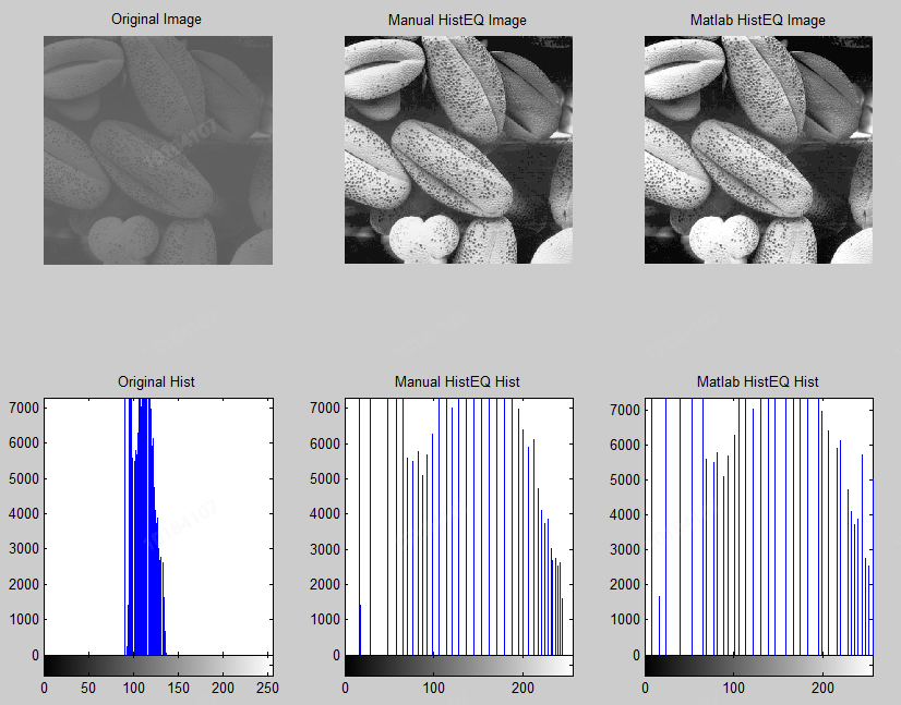
As shown in the figure above, it is the result of image equalization of the original image and the source code / matlab image library. The results are similar to the comparison chart, but the histogram is still slightly different. The main reason is that we have adopted the fixed-point method, and the error is within the tolerable range.
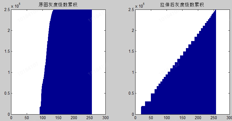
Finally, check the gray level series accumulation diagram before and after histogram equalization, as shown below. We can see that the gray level in the original image is concentrated and distributed. After re equalization, the gray level series increases within 0-255. Therefore, the effect of gray level stretching is achieved, the contrast and recognition of the image are enhanced, and the requirements of this article are met.
4. FPGA implementation of histogram equalization
To be continued, please look forward to
Disadvantages of histogram equalization:
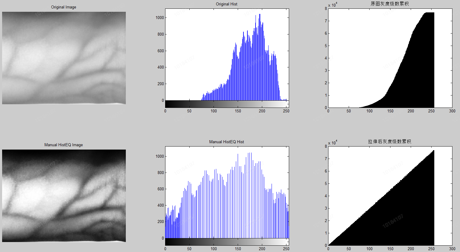
If an image is dark or bright as a whole, the histogram equalization method is very suitable. For example, in vein recognition, the image collected by the camera after 850 nm infrared exposure will be a little darker in order to prevent overexposure and loss of information. Then the image enhancement effect can be achieved simply and quickly after histogram equalization, which increases the recognition degree of subsequent algorithms, as shown in the following figure:
However, histogram equalization is a global processing method. It does not select the processed data, which may increase the contrast of background interference information and reduce the contrast of useful signals, resulting in image abnormalities. Therefore, it mainly has the following disadvantages:
1) After transformation, the gray level of the image is reduced and some details are lost
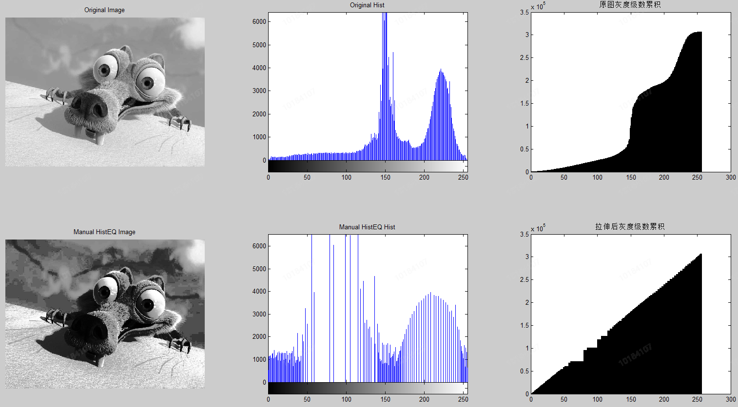
2) The peak of histogram is the unnatural excessive enhancement of contrast after stretching.
For example, in the following images, the image contrast is enhanced after contrast stretching. Although the gray level increases linearly after stretching, it causes local darkness or overexposure, resulting in abnormal image and loss of many details, but the gain is not worth the loss.
Therefore, the local histogram equalization method can solve the problem of anomalies caused by global image processing. Further in-depth research is left to the readers. This film is over.
Because histogram equalization is realized in gray domain, it mainly aims at brightness stretching, and RGB image has three channels of data. Histogram stretching can be carried out on three channels respectively, but this may cause image color distortion. Therefore, it can be converted to YCbCr format, histogram equalization of Y, and then back to RGB format.
Matlab digital image processing - Gonzalez Gallery download address:
http://www.imageprocessingplace.com/DIP-3E/dip3e_book_images_downloads.htm
reference:
https://blog.csdn.net/charlene_bo/article/details/70263344?utm_source=blogxgwz3
https://blog.csdn.net/qq_15971883/article/details/88699218
I am CrazyBingo!
This article is a chapter in the course of image acceleration based on Matlab and FPGA. Before the official publication, I will take the lead in official account / blog to share with you. Please be bold in correcting!!!