1. Introduction of convolutional neural network
Convolutional neural network (CNN), the earliest one was in 1860's. biologists found that each visual neuron can only process a small area of visual image, that is, the receptive field. Later, in the 1980s, Japanese scientists put forward the concept of neurocognitron, which can also be regarded as the initial prototype of convolutional neural network. In CS231n class, they said that convolutional neural network was not produced overnight. From this development process, we can see that it is indeed so. The main points of convolutional neural network are Local Connection, Weight sharing and down sampling in Pooling layer.  
2. Construction of simple neural network
Here we use two convolution layers and a full connection layer to explain how to define the convolution layer and the full connection layer in tensorflow.

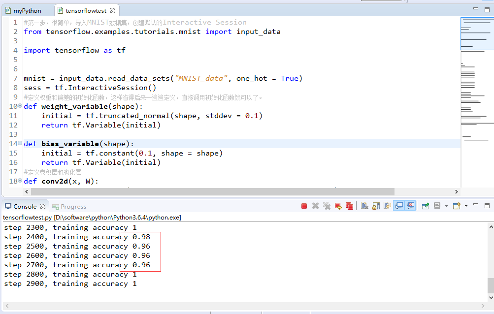
#The first step is to import the MNIST data set and create the default Interactive Session
from tensorflow.examples.tutorials.mnist import input_data

import tensorflow as tf


mnist = input_data.read_data_sets("MNIST_data", one_hot = True)
sess = tf.InteractiveSession()
#Define the initialization function of weight and deviation, so as to save the subsequent definition over and over, and directly call the initialization function.
def weight_variable(shape):
    initial = tf.truncated_normal(shape, stddev = 0.1)
    return tf.Variable(initial)

def bias_variable(shape):
    initial = tf.constant(0.1, shape = shape)
    return tf.Variable(initial)
#Define the convolution layer and pooling layer
def conv2d(x, W):
    return tf.nn.conv2d(x, W, strides = [1, 1, 1, 1], padding = 'SAME')

def max_pool_2_2(x):
    return tf.nn.max_pool(x, ksize = [1, 2, 2, 1], strides = [1, 2, 2, 1], padding = 'SAME')

'''
//Define the placeholder of the input, x is the feature, y ﹣ is the real label. Because convolutional neural networks use 2D spatial information,
//So to restore 784 dimension data to 28 * 28 structure, the function used is tf.shape.
'''
x = tf.placeholder(tf.float32, [None, 784])
y_ = tf.placeholder(tf.float32, [None, 10])
x_image = tf.reshape(x, [-1, 28, 28, 1])

#First convolutional nerve
W_conv1 = weight_variable([5, 5, 1, 32])
b_conv1 = bias_variable([32])
h_conv1 = tf.nn.relu(conv2d(x_image, W_conv1) + b_conv1)
h_pool1 = max_pool_2_2(h_conv1)

#The second convolution nerve
W_conv2 = weight_variable([5, 5, 32, 64])
b_conv2 = bias_variable([64])
h_conv2 = tf.nn.relu(conv2d(h_pool1, W_conv2) + b_conv2)
h_pool2 = max_pool_2_2(h_conv2)

#Define the first full connection layer
W_fc1 = weight_variable([7 * 7 * 64, 1024])
b_fc1 = bias_variable([1024])
h_pool2_flat = tf.reshape(h_pool2, [-1, 7 * 7 * 64])
h_fc1 = tf.nn.relu(tf.matmul(h_pool2_flat, W_fc1) + b_fc1)

keep_prob = tf.placeholder(tf.float32)
h_fc1_drop = tf.nn.dropout(h_fc1, keep_prob)

#The final output layer also initializes the weights and deviations.
W_fc2 = weight_variable([1024, 10])
b_fc2 = bias_variable([10])
y_conv = tf.nn.softmax(tf.matmul(h_fc1_drop, W_fc2) + b_fc2)

#Define the loss function and training steps, and use the Adam optimizer to minimize the loss function.
cross_entropy = tf.reduce_mean(-tf.reduce_sum(y_ * tf.log(y_conv), reduction_indices = [1]))
train_step = tf.train.AdamOptimizer(1e-4).minimize(cross_entropy)

#Calculate the accuracy of the forecast.
correct_prediction = tf.equal(tf.argmax(y_conv, 1), tf.argmax(y_, 1))
accuracy = tf.reduce_mean(tf.cast(correct_prediction, tf.float32))

'''
//Initialization of global variables, 20000 iterations of training, using 50 minibatch, so the total number of training samples is 1 million.
'''
tf.global_variables_initializer().run()
for i in range(20000):
    batch = mnist.train.next_batch(50)
    if i % 100 == 0:
        train_accuracy = accuracy.eval(feed_dict = {x: batch[0], y_: batch[1], keep_prob: 1.0})
        print("step %d, training accuracy %g"%(i, train_accuracy))
    train_step.run(feed_dict = {x: batch[0], y_: batch[1], keep_prob: 0.5})

#Output the final accuracy.
print("test accuracy %g"%accuracy.eval(feed_dict = {x: mnist.test.images, y_: mnist.test.labels, keep_prob: 1.0}))