Original link: http://tecdat.cn/?p=2687
Original source: Tuo end data tribal official account
What is MCMC and when to use it?
MCMC is just an algorithm for sampling from distribution.
This is just one of many algorithms. This term stands for "Markov chain Monte Carlo" because it is a "Monte Carlo" (i.e. random) method using "Markov chain" (we will discuss later). MCMC is only one kind of Monte Carlo method, although many other common methods can be regarded as simple special cases of MCMC.
Why should I sample from the distribution?
Sampling from the distribution is the simplest way to solve some problems.
Perhaps the most common method of MCMC is to extract samples from the posterior probability distribution of a model in Bayesian reasoning. Through these samples, you can ask some questions: "what is the average value and reliability of the parameters?".
If these samples are independent samples from the distribution, the estimated mean will converge to the real mean.
Suppose our target distribution is a normal distribution s with mean m and standard deviation.
As an example, consider using the mean m and the standard deviation s to estimate the mean of the normal distribution (here, I will use the parameters corresponding to the standard normal distribution):
We can easily use this rnorm function to sample from this distribution
seasamples<-rn 000,m,s)
The average value of the sample is very close to the real average (zero):
 mean(sa es)

 ## \[1\] -0. 537
In fact, in this case, the expected variance of the $n $sample estimate is $1 / n $, so we expect most of the values to be $\ pm 2 \, / \ sqrt {n} = 0.02.
 summary(re 0,mean(rnorm(10000,m,s))))

 ## Min. 1st Qu. Median Mean 3rd Qu. Max.
## -0.03250 -0.00580 0.00046 0.00042 0.00673 0.03550
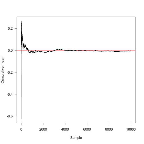
This function calculates the sum of the cumulative averages.
 cummean<-fun msum(x)/seq_along(x)

 plot(cummaaSample",ylab="Cumulative mean",panel.aabline(h=0,col="red"),las=1)
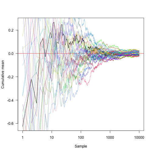
Convert the x-axis to logarithmic coordinates and display another 30 random methods:
Sample quantiles can be extracted from your series of sampling points.
This is the point of analysis and calculation, and its probability density of 2.5% is lower than:
 p<-0.025

a.true<-qnorm(p,m,s)

a.true

1## \[1\] -1.96
We can estimate this by direct integration in this case
aion(x)
dnorm(x,m,s)
g<-function(a)
integrate(f,-Inf,a)$value
a.int<-uniroot(function(x)g(a10,0))$roota.int

1## \[1\] -1.96
Monte Carlo integration is used to estimate the points:
a.mc<-unnasamples,p))
a.mc

## \[1\] -2.023

a.true-a.mc

## \[1\] 0.06329
However, within the limit where the sample size tends to infinity, this will converge. In addition, it is possible to make a statement on the nature of the error; If we repeat the sampling process 100 times, we get a series of estimates of errors with the same amplitude as the errors near the mean:
 a.mc<-replicate(anorm(10000,m,s),p))
summary(a.true-a.mc)
 ## Min. 1st Qu. Median Mean 3rd Qu. Max.
## -0.05840 -0.01640 -0.00572 -0.00024 0.01400 0.07880
This kind of thing is really common. In most Bayesian reasoning, a posteriori distribution is a function of some (possibly large) parameter vectors, and you want to reason about a subset of these parameters.
In a hierarchical model, you may have a large number of random effects fitted, but you most want to infer a parameter. stay
In the Bayesian framework, you can calculate the marginal distribution of the parameters you are interested in on all other parameters (this is what we want to do above).
Why does "traditional statistics" not use Monte Carlo method?
For many problems in traditional teaching statistics, instead of sampling from the distribution, the function can be maximized or maximized. So we need some functions to describe the possibility and maximize it (maximum likelihood reasoning), or some functions to calculate the sum of squares and minimize it.
However, the function of Monte Carlo method in Bayesian statistics is the same as that in frequency statistics, which is only an algorithm for reasoning. So once you basically know what MCMC is doing, you can treat it like most people treat their optimizer as a black box, like a black box.
Markov chain Monte Carlo
Suppose we want to extract some target distributions, but we can't extract independent samples as before. There is a solution using Markov chain Monte Carlo (MCMC) to do this. First, we must define something so that the next sentence makes sense: what we have to do is try to construct a Markov chain, which samples the target distribution as its stable distribution.
definition
Suppose we have a three state Markov process. Let P be the transition probability matrix in the chain:
 P<-rbind(a(.2,.1,.7),c(.25,.25,.5))
P

 ## \[,1\] \[,2\] \[,3\]
## \[1,\] 0.50 0.25 0.25
## \[2,\] 0.20 0.10 0.70
## \[3,\] 0.25 0.25 0.50

 rowSums(P)

 ## \[1\] 1 1 1
P[i,j] gives the probability j from state i to state.
Note that unlike rows, columns do not necessarily sum to 1:
 colSums(P)

 ## \[1\] 0.95 0.60 1.45
This function takes a state vector x (where x[i] is the probability I of being in a state) and iterates it P by multiplying it by the transition matrix, so that the system proceeds to step n.
 iterate.P<-function(x,P,n){
res<-matrix(NA,n+1,len
a<-xfor(iinseq_len(n))
res\[i+1,\]<-x<-x%*%P
res}
Start with the system in state 1 (the same is true for the x vector [1,0,0], indicating that the probability of being in state 1 is 100% and not in any other state)
Similarly, for the other two possible starting states:
 y2<-iterate.P(c(0,1,0),P,n)
y3<-iterate.P(c(0,0,1),P,n)
This shows the convergence of stationary distribution.
ma=1,xlab="Step",ylab="y",las=1)
matlines(0:n,y2,lty=2)
matlines(0:n,y3,lty=3)
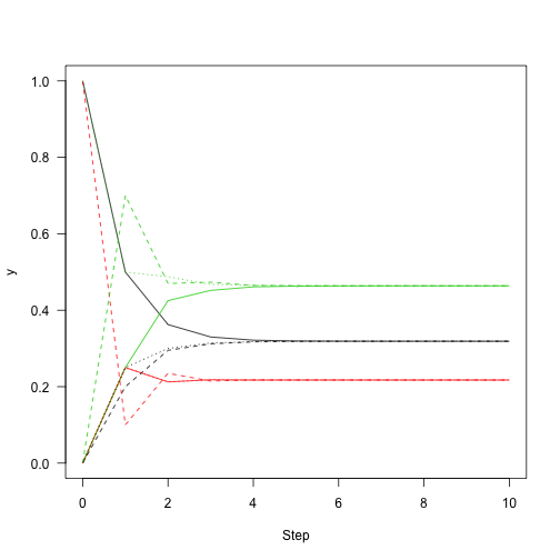
We can use the eigen function of R to extract the main eigenvector of the system (t() here transpose the matrix to get the left eigenvector).
 v<-eigen(t(P)
ars\[,1\]
v<-v/sum(v)#Normalized eigenvector
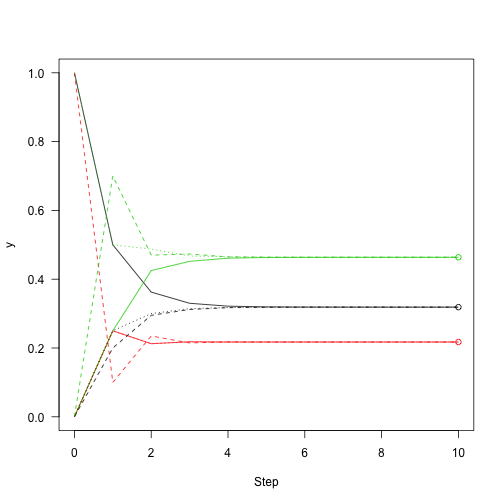
Then add a point to the previous number to show how close we are to convergence:
matplot(0:n,y1a3,lty=3)
points(rep(10,3),v,col=1:3)
The above process iterates the overall probability of different states; Not through the actual conversion of the system. So let's iterate the system, not the probability vector.
run<-function(i,P,n){
res<-integer(n)
for(a(n))
res\[\[t\]\]<-i<-sample(nrow(P),1,pr=P\[i,\])
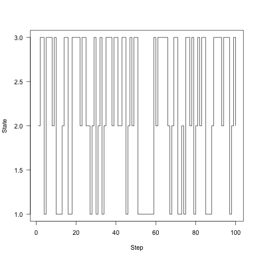
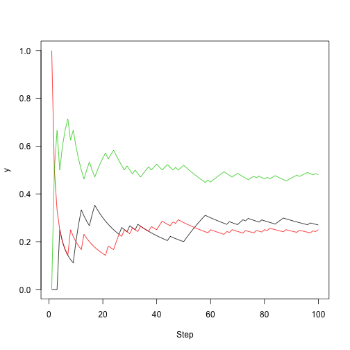
res}The chain runs 100 steps:
 samples<-run(1,P,100)
ploaes,type="s",xlab="Step",ylab="State",las=1)
Instead of plotting States, plot our time fraction over time in each state:
 plot(cummean(samplesa2)
lines(cummean(samples==3),col=3)
Run again (5000 steps)
 n<-5000
set.seed(1)
samples<-run(1,P,n)
plot(cummeanasamples==2),col=2)
lines(cummean(samples==3),col=3)
abline(h=v,lty=2,col=1:3)
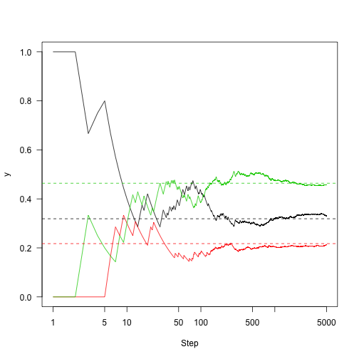
So the key here is: Markov chains have some good properties. Markov chains have a fixed distribution. If we run them long enough, we can see where the chain spends time and reasonably estimate the stationary distribution.
Metropolis algorithm
This is the simplest MCMC algorithm.
MCMC sampling 1d (single parameter) problem
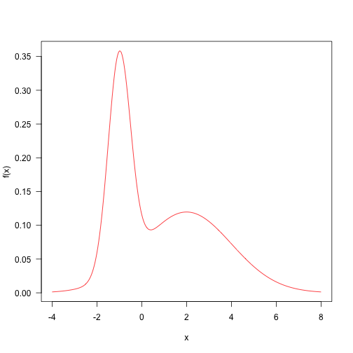
This is the weighted sum of two normal distributions. This distribution is quite simple and samples can be taken from MCMC.
Here are some definitions of parameters and target density.
 p<-0.4ma1,2)
sd<-c(.5,2)
f<-function(x)p\*dnora\],sd\[1\])+(1-p)\*dnorm(x,mu\[2\],sd\[2\])
Probability density mapping
Let's define a very simple algorithm that samples from a normal distribution with a standard deviation of 4 centered on the current point
This requires only a few steps of running MCMC. It will return a matrix from point x with the same number of nsteps rows and columns as the number of columns of the X element. If you run on a scalar, x it returns a vector.
 run<-funagth(x))
for(iinseq_len(nsteps))
res\[i,\]<-x<-step(x,f,q)
drop(res)}
Here is the first 1000 steps of Markov chain, and the target density is on the right:
 layout(matrix(ca,type="s",xpd=NA,ylab="Parameter",xlab="Sample",las=1)
usr<-par("usr")
xx<-seq(usr\[a4\],length=301)
plot(f(xx),xx,type="l",yaxs="i",axes=FALSE,xlab="")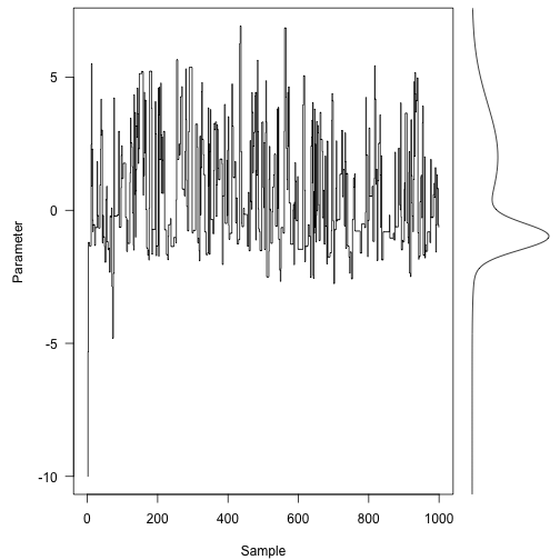
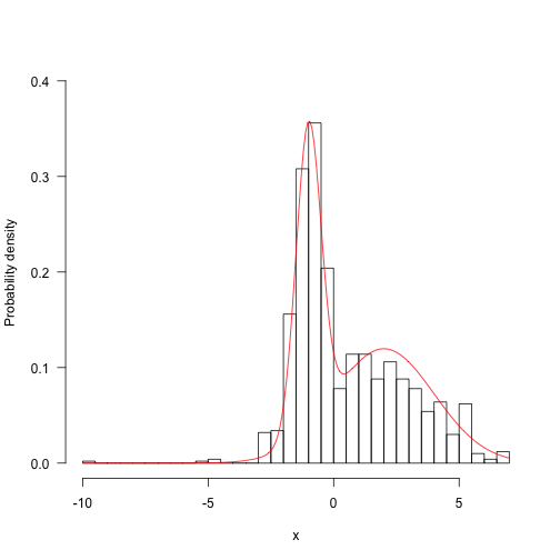
hist(res,5aALSE,main="",ylim=c(0,.4),las=1,xlab="x",ylab="Probability density")
z<-integrate(f,-Inf,Inf)$valuecurve(f(x)/z,add=TRUE,col="red",n=200)
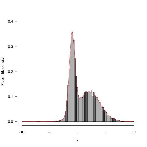
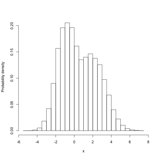
Run longer and the results begin to look better:
res.long<-run(-10,f,q,50000)
hist(res.long,100,freq=FALSE,main="",ylim=c(0,.4),las=1,xlab
Now, run different scenarios - one with a large standard deviation (33) and the other with a small standard deviation (3).
res.fast<-run(-10action(x)
rnorm(1,x,33),1000)
res.slow<-run(-10,f,functanorm(1,x,.3),1000)
Notice how the three tracks are moving.
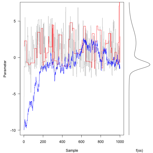
On the contrary, the red trace rejects most of the space.
The blue trail suggests small movements that tend to be accepted, but it walks randomly with most of the tracks. It takes hundreds of iterations to reach most of the probability density.
You can see the effect of different scheme steps in autocorrelation in the subsequent parameters - these figures show the attenuation of autocorrelation coefficient between different lag steps, and the blue line indicates statistical independence.
 par(mfrow=c(1,3ain="Intermediate")
acf(res.fast,las=1,m
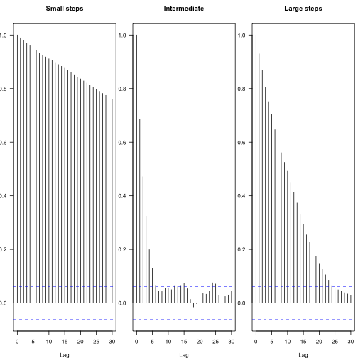
Thus, the effective number of independent samples can be calculated:
1coda::effectiveSize(res)

1 2## var1 ## 187

1coda::effectiveSize(res.fast)

1 2## var1 ## 33.19

1coda::effectiveSize(res.slow)

1 2## var1 ## 5.378
This more clearly shows that the chain runs longer:
 naun(-10,f,q,n))
xlim<-range(sapply(saa100)
hh<-lapply(samples,function(x)
hist(x,br,plot=FALSE))
ylim<-c(0,max(f(xx)))
Display 100, 1000, 10000 and 100000 steps:
for(hinhh){plot(h,main="",freq=a=300)}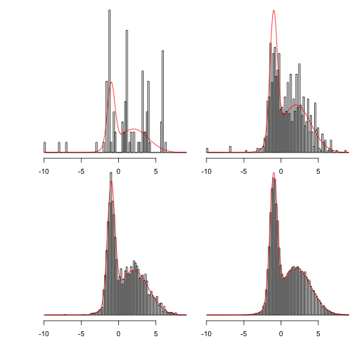
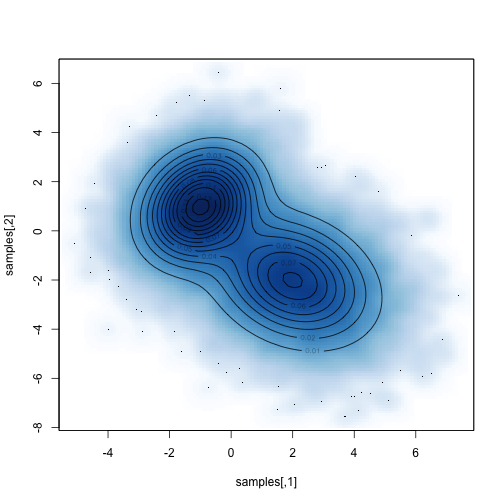
MCMC in two dimensions
A multivariate normal density is given, and a mean vector (center of distribution) and variance covariance matrix are given.
make.mvn<-function(mean,vcv){
logdet<-as.numeric(detea+logdet
vcv.i<-solve(vcv)function(x){
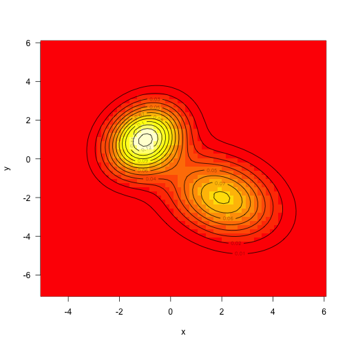
dx<-x-meanexp(-(tmp+rowSums((dx%*%vcv.i)*dx))/2)}}As mentioned above, the target density is defined as the sum of two mvns (unweighted this time):
 mu1<-c(-1,1)mu2<-c(2,-2)
vcv1<-ma5,.25,1.5),2,2)
vcv2<-matrix(c(2,-.5,-.5,2aunctioax)+f2(x)x<-seq(-5,6,length=71)
y<-seq(-7,6,lena-expand.grid(x=x,y=y)
z<-matrix(aaTRUE)
Sampling from multivariate normal distribution is also quite simple, but we will use MCMC to extract samples from it.
Here are some different strategies - we can propose actions in two dimensions at the same time, or we can sample along each axis independently. Both strategies work, although their mixing speed will be different.
Assuming we don't actually know how to sample from mvn, let's propose a consistent proposal distribution in two dimensions, sampling from a square with a width of "d" on each side.
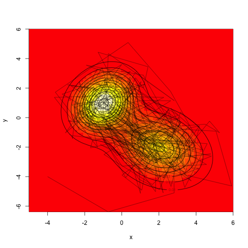
Compare the sampling distribution with the known distribution:
For example, what is the marginal distribution of parameter 1?
hisales\[,1\],freq=FALSa",xlab="x",ylab="Probability density")
We need to integrate all possible values of the second parameter of the first parameter. Then, because the objective function itself is not standardized, we must decompose it into one-dimensional integral values.
 m<-function(x1){
g<-Vectorize(function(x2)f(c(x1,ae(g,-Inf,Inf)$value}
xx<-seq(mina\]),max(sales\[,1\]),length=201)
yy<-s
ue
hist(samples\[,1\],freq=FALSE,ma,0.25))
lines(xx,yy/z,col="red")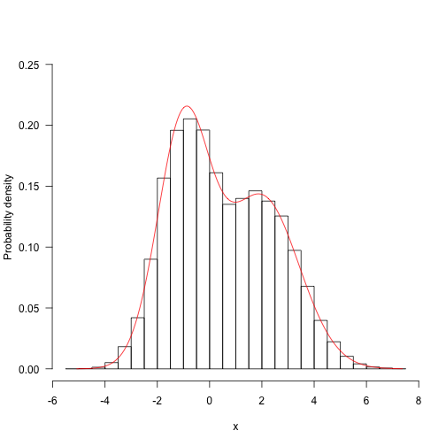

Most popular insights
1.Markov Regime Switching Model in R language Model ")
2.Implementation of Markov chain Monte Carlo MCMC model in R language
3.matlab Bayesian hidden Markov hmm model
4.Using machine learning to identify changing stock market conditions -- Application of hidden Markov model (HMM) Application of ")
5.R language hidden Markov model hmm identifies changing market conditions
6.Implementation of hidden Markov model (HMM) in matlab Implementation ")
7.Realizing Markov switching ARMA – GARCH model of MCMC with matlab
8.How to make markov switching model in R language
9.Research on traffic casualties based on R language Markov transformation model