Probabilistic representation of CBOW model:

P(A): probability of occurrence of A.

P(A,B): the probability of simultaneous occurrence of event A and event B, which is called joint probability.

P(A|B): the probability of event A after giving the information of event B, which is called A posteriori probability.

CBOW model: the probability of outputting the target word when a context is given.

The probability that the target word is wt given the context wt-1 and wt+1 is expressed by a mathematical formula:

Cross entropy error function formula: yk is the output of neural network, tk is the correct solution label, and k represents the dimension of data. If the tag is one hot, that is, only the correct unlabeled index in tk is 1, and the others are 0. Then the formula only calculates the natural logarithm of the output corresponding to the correct solution label.

Loss function of CBOW model (loss function of one sample data):

Loss function of CBOW model (extended to the whole corpus):

The task of CBOW model learning: make the above loss function as small as possible. At that time, the weight parameter is the distributed representation of the desired word. (only the case where the window size is 1 is considered here)

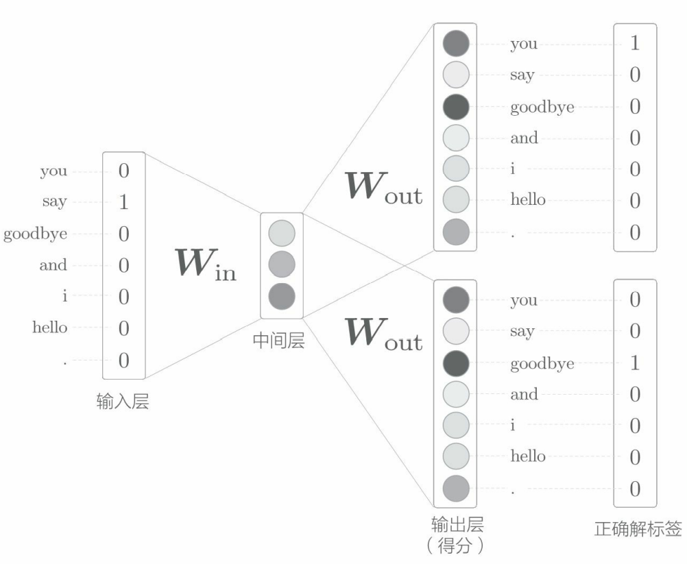
Skip gram model: CBOW model predicts the middle word (target word) from multiple words in the context, while skip gram model predicts multiple surrounding words (context) from the middle word (target word).

The network structure of skip gram model: there is only one input layer, and the number of output layers is equal to the number of words in the context. The loss of each output layer (through the Softmax with Loss layer, etc.) shall be calculated separately, and then they shall be added up as the final loss.

Mathematical representation of skip gram model:

In the skip gram model, conditional independence is assumed between words in the context.

By substituting the cross entropy error function, the loss function of a sample data of skip gram model can be derived. The loss function of skip gram model first calculates the losses corresponding to each context, and then adds them together.

Extended to the whole corpus, the loss function of skip gram model can be expressed as:

Skip gram is more accurate than CBOW. CBOW model is faster than skip gram model.

Implementation of skip gram model:

import sys
sys.path.append('..')
import numpy as np
from common.layers import MatMul, SoftmaxWithLoss


class SimpleSkipGram:
    def __init__(self, vocab_size, hidden_size):
        V, H = vocab_size, hidden_size

        # Initialize weight
        W_in = 0.01 * np.random.randn(V, H).astype('f')
        W_out = 0.01 * np.random.randn(H, V).astype('f')

        # Generation layer
        self.in_layer = MatMul(W_in)
        self.out_layer = MatMul(W_out)
        self.loss_layer1 = SoftmaxWithLoss()
        self.loss_layer2 = SoftmaxWithLoss()

        # Organize all weights and gradients into a list
        layers = [self.in_layer, self.out_layer]
        self.params, self.grads = [], []
        for layer in layers:
            self.params += layer.params
            self.grads += layer.grads

        # Set the distributed representation of the word as a member variable
        self.word_vecs = W_in

    def forward(self, contexts, target):
        h = self.in_layer.forward(target)
        s = self.out_layer.forward(h)
        l1 = self.loss_layer1.forward(s, contexts[:, 0])
        l2 = self.loss_layer2.forward(s, contexts[:, 1])
        loss = l1 + l2
        return loss

    def backward(self, dout=1):
        dl1 = self.loss_layer1.backward(dout)
        dl2 = self.loss_layer2.backward(dout)
        ds = dl1 + dl2
        dh = self.out_layer.backward(ds)
        self.in_layer.backward(dh)
        return None

Call this skip gram model

# coding: utf-8
import sys
sys.path.append('..')  # Settings for importing files from the parent directory
from common.trainer import Trainer
from common.optimizer import Adam
#from simple_cbow import SimpleCBOW
from simple_skip_gram import SimpleSkipGram
from common.util import preprocess, create_contexts_target, convert_one_hot


window_size = 1
hidden_size = 5
batch_size = 3
max_epoch = 1000

text = 'You say goodbye and I say hello.'
corpus, word_to_id, id_to_word = preprocess(text)

vocab_size = len(word_to_id)
contexts, target = create_contexts_target(corpus, window_size)
target = convert_one_hot(target, vocab_size)
contexts = convert_one_hot(contexts, vocab_size)

#model = SimpleCBOW(vocab_size, hidden_size)
model = SimpleSkipGram(vocab_size, hidden_size)
optimizer = Adam()
trainer = Trainer(model, optimizer)

trainer.fit(contexts, target, max_epoch, batch_size)
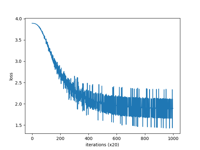
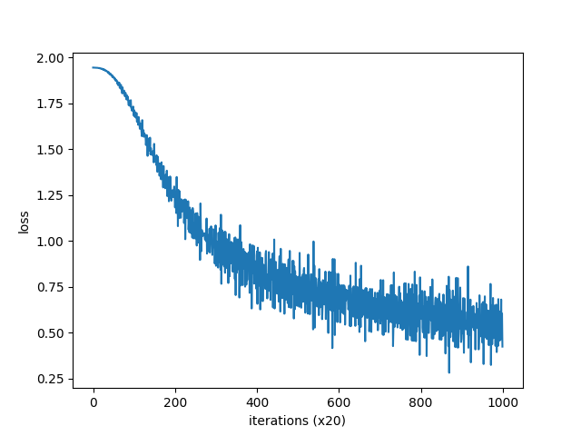
trainer.plot()

word_vecs = model.word_vecs
for word_id, word in id_to_word.items():
    print(word, word_vecs[word_id])

you [ 0.0070119   0.01140655 -0.00602617 -0.00951831  0.00306297]
say [ 0.90311    -0.90883684  0.92998946  0.9578707   1.1098603 ]
goodbye [-0.8135963   0.805687   -0.8332484  -0.86875284  1.1370432 ]
and [ 0.9542584  -0.9512509   0.97993344  0.98317575 -1.2883114 ]
i [-0.80985945  0.81495476 -0.85571784 -0.84448576  1.1391366 ]
hello [-0.8404988  0.8455065 -0.8266616 -0.8118625 -1.3357102]
. [-0.01073505 -0.01199387 -0.02076071 -0.01374857  0.01593136]

Compare the output of the previous CBOW model: it is found that the dense vector representation of words obtained by the two methods is very different.

you [-0.9987413   1.0136298  -1.4921554   0.97300434  1.0181936 ]
say [ 1.161595   -1.1513934  -0.25779223 -1.1773298  -1.1531342 ]
goodbye [-0.88470864  0.9155085  -0.30859873  0.9318609   0.9092796 ]
and [ 0.7929211 -0.8148116 -1.8787507 -0.7845257 -0.8028278]
i [-0.8925459   0.95505357 -0.29667985  0.90895575  0.90703803]
hello [-1.0259517   0.97562104 -1.5057516   0.96239203  1.0297285 ]
. [ 1.2134467 -1.1766206  1.6439314 -1.1993438 -1.1676227]