Introduction: This article will explore some practical knowledge related to statistics of Scipy package. The intention is to explore some basic methods of statistical analysis and the corresponding Python implementation methods. Combining theory with practice, this paper vividly expresses the boring statistical knowledge through practical stock market data, which is convenient for everyone to understand at a glance and use it immediately!

Statistics is a science of collecting, processing, analyzing, interpreting data and drawing conclusions from it. Its core is data.
The four steps of data analysis are data collection → data processing → data analysis → data interpretation.
There are two methods for statistical analysis of data:
- Descriptive analysis methods: overall scale, comparison relationship, concentration trend, dispersion degree, skewness, kurtosis
- Inferential analysis methods estimation, hypothesis test, contingency analysis, analysis of variance, correlation analysis, regression analysis
The official account of this article is only part of the core code. This article provides a complete version of PDF Download with full code. The way to get it is to pay attention to the public number "data STUDIO" and reply to [210512] access. If you are not interested in the code, skip it directly without affecting your reading.
modular
This paper mainly realizes statistical distribution and test based on SciPy. SciPy is based on NumPy and provides more scientific computing functions, such as linear algebra, optimization, integration, interpolation, signal processing, etc.
The functions of Scipy include optimization, linear algebra, integration, interpolation, fitting, special functions, fast Fourier transform, signal processing and image processing, ordinary differential equation solving and other calculations commonly used in science and engineering, and these functions are needed for data analysis later.
import seaborn as sns
from scipy import stats
from scipy.stats import norm
import math
Data preparation
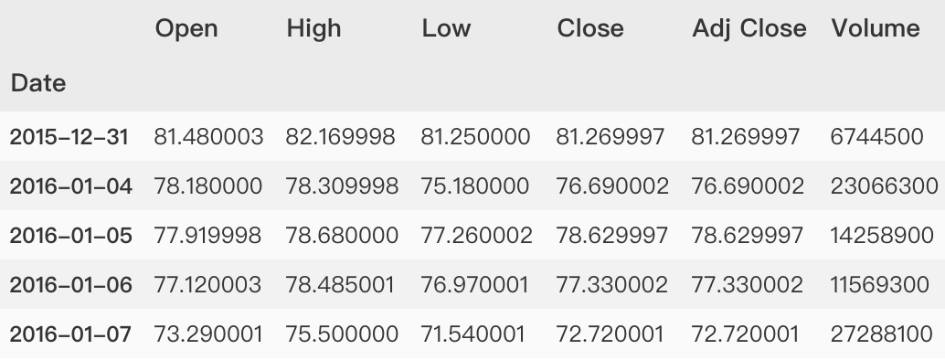
This paper will continue to use the financial stock market data, market = 'TCEHY' and symbol = 'BABA' stock market data. Please refer to the relevant acquisition methods Financial stock market data preparation . The sample data is shown below.
Feature creation
- Covariance matrix
It consists of the covariance of two variables in the data set. Second order of matrix
(i,j)The first element is the second element in the dataset
iAnd section
jCovariance of elements.
- Covariance
It is to measure the synchronization degree of the changes of two variables, that is, to measure the linear correlation degree of two variables. If the covariance of the two variables is 0, they are statistically considered to be linearly independent. Note that two unrelated variables are not completely independent, but there is no linear correlation.
new_df = pd.DataFrame(
          {symbol : df['Adj Close'],
           market : dfm['Adj Close']},
          index=df.index)
# Calculate rate of return
new_df[['stock_returns',
        'market_returns']] = new_df[[symbol,market]] / new_df[[symbol,market]].shift(1) -1
new_df = new_df.dropna()
# np.cov() estimates the covariance matrix for a given data and weight
# Covariance is used to measure the overall error of two variables
covmat = np.cov(new_df["stock_returns"],
                new_df["market_returns"])
# calculation
beta = covmat[0,1]/covmat[1,1]
alpha= np.mean(new_df["stock_returns"]
              )-beta*np.mean(new_df["market_returns"])
In order to understand the above calculation, print some results and have a look.
>>> print(covmat)
[[0.00044348 0.00027564]
[0.00027564 0.00042031]]'
>>> print('Beta:', beta)
Beta: 0.6558020316481588'
>>> print('Alpha:', alpha)
Alpha: 0.00023645436856520742'
statistical analysis
Take the field 'Adj Close' as an example
close = df['Adj Close']
Mean value
The quantity indicating the trend in a set of data refers to the sum of all data in a set of data divided by the number of this set of data.
np.mean(close)
163.4495238561479
Median
The number in the middle of a set of data arranged in order.
np.median(close)
172.54000091552734
Mode mode
It refers to the value with obvious centralized trend points in the statistical distribution, representing the general level of data. It is also the most frequent value in a group of data. Sometimes there are several modes in a group of numbers.
mode = stats.mode(close)
print("The median is {} Count as {}".format(mode.mode[0], mode.count[0]))
The median is 67.02999877929688 The count is 2
Range full range
Full range is also called "range". It is the difference between the maximum and minimum values in a set of data. It can be used to measure the dispersion of data.
np.ptp(close)
256.5700149536133
Variance variance
In statistical description, variance is used to calculate the difference between each variable (observed value) and the overall mean.
np.var(close)
3185.8517317644914
Standard deviation
The square root of variance, which is used to measure how data is dispersed.
np.std(close)
56.443349756764896
Standard error
The standard deviation is the arithmetic square root of variance and estimates the variability between sample means. The standard deviation can reflect the dispersion of a data set. If the mean is the same, the standard deviation may not be the same.
stats.sem(close)
1.5907426123008535
Z-Scores
The observed value is obtained by subtracting the average value of the group of observed values and dividing it by the standard deviation, indicating how many standard deviations the element is far from the mean value.
znp.abs(stats.zscore(close))
[1.45596474 1.53710795 1.50273729 ...
  1.2899743  1.32771134 1.22743374]
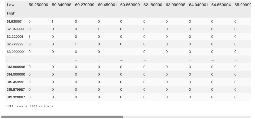
Continuity table Contingency Table
The contingency table shows the correlation between the two variables.
pd.crosstab(df['High'],
            df['Low'],
            margins = False)
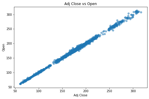
Scatter plot
Scatter diagram refers to the distribution diagram of data points on the plane of rectangular coordinate system in regression analysis. The scatter diagram represents the general trend of dependent variables changing with independent variables. Therefore, an appropriate function can be selected to fit the data points.
plt.scatter(df['Adj Close'],
            df['Open'], alpha=0.5)
Regression
Regression is the study of a set of random variables(
Y_1 ,Y_2 ,...,Y_i)And another group(
X_1,X_2,...,X_k)The statistical analysis method of the relationship between variables is also called multiple regression analysis. It measures the relationship between the average value of one variable and the corresponding value of other variables.
from sklearn.linear_model import LinearRegression
X = np.array(df['Open']).reshape(df.shape[0],-1)
y = np.array(df['Adj Close'])
LR = LinearRegression().fit(X, y)
# Some properties
LR.score(X, y)
LR.coef_
LR.intercept_
LR.predict(X)
Prediction results of elementary probability theory
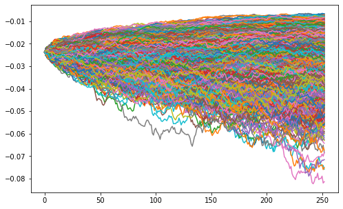
Monte Carlo method
It is an experimental calculation algorithm based on repeated random samples.
df['Returns'] = df['Adj Close'].pct_change()
df['Returns'] = df['Returns'].dropna()
df = df.dropna()

S = df['Returns'][-1]     # Initial stock price
T = 252                   # Transaction days
mu = df['Returns'].mean() # mean value
sigma = df['Returns'].std()*math.sqrt(252) #amplitude
Random variables and probability distribution
Common stock probability distribution methods [1]
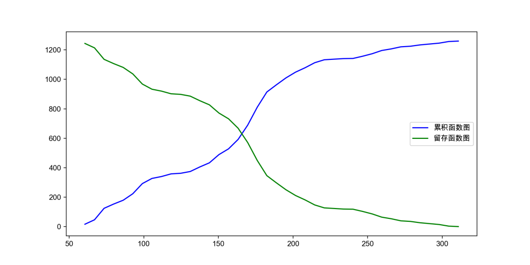
Cumulative distribution
Cumulative Distribution Function, also known as distribution function, is the integral of probability density function, which can completely describe the probability distribution of a real random variable X. Generally, it is marked with capital "CDF" (Cumulative Distribution Function).
The cumulative distribution diagram is a distribution diagram of the frequency or rate of the measured value less than a certain value to the group limit when grouped according to a certain group.
There are two drawing methods in matplotlib
- plt.plot()
- plt.step()
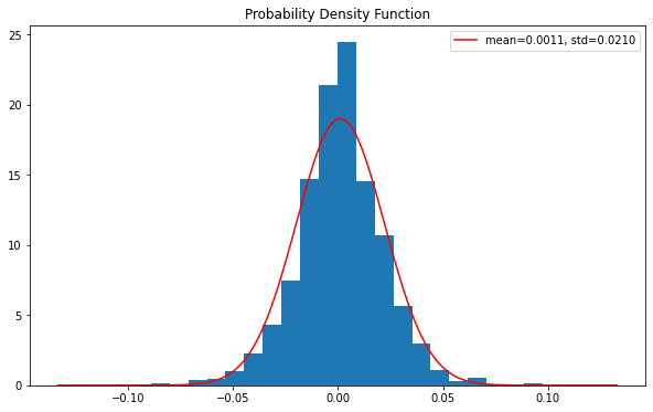
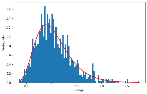
probability density function
Probability density function (PDF) is a continuous random variable with the value of a given sample in the sample space, which can be interpreted as providing the relative possibility that the value of the random variable is equal to the value of the sample.
values = df['Returns'][1:]
x = np.linspace(values.min(), values.max(), len(values))
loc, scale = stats.norm.fit(values)
param_density = stats.norm.pdf(x, loc=loc, scale=scale)
ax.hist(values, bins=30, density=True)
ax.plot(x, param_density, 'r-', label=label)
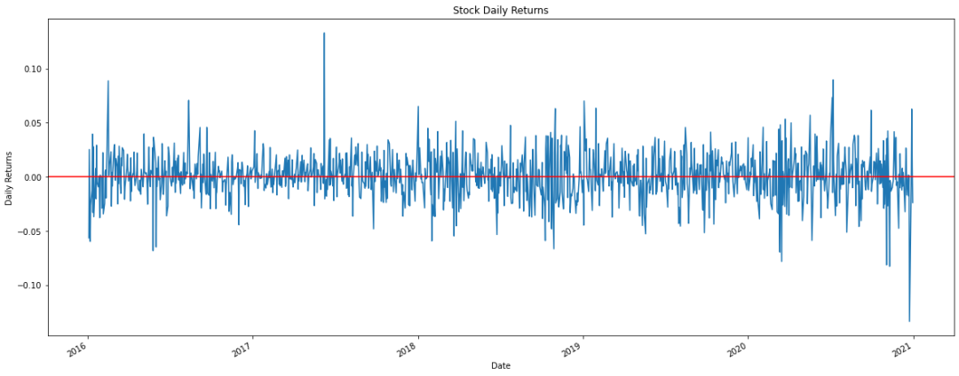
# At this stage, the rate of return rises and falls
df['Returns'].plot(figsize=(20, 8))
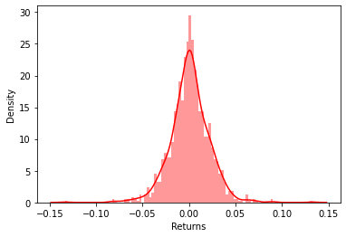
seaborn draws histogram: divide boxes first, and then calculate the data distribution of each box division frequency.
sns.distplot(df['Returns'].dropna(),bins=100,color='red')
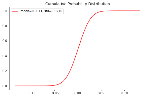
Cumulative probability distribution
Cumulative probability distribution, also known as cumulative distribution function, distribution function, etc., is used to describe the probability of random variables falling on any interval. It is often regarded as a certain feature of data.
If the variable is a continuous variable, the cumulative probability distribution is a function obtained by integrating the probability density function.
If the variable is a discrete variable, the cumulative probability distribution is a function obtained by the addition of the distribution law.
param_density = stats.norm.cdf(x, loc=loc, scale=scale)
ax.plot(x, param_density, 'r-', label=label)
uniform distribution
It is a symmetric probability distribution, and the distribution probability at the same length interval is equally possible.
The uniform distribution belongs to the continuous probability distribution function, and the default is the uniform distribution of [0,1].
values = df['Returns'][1:]
s = np.random.uniform(values.min(), values.max(), len(values))
# s = scipy.stats.uniform(loc=values.min(),
#     scale=values.max()-values.min())
count, bins, ignored = plt.hist(s, 15, density=True)
plt.plot(bins, np.ones_like(bins), linewidth=2, color='r')
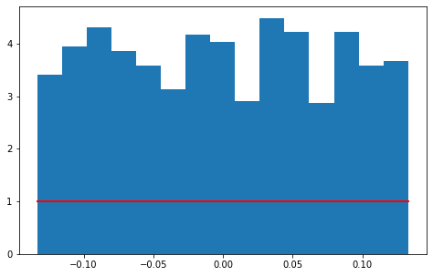
np.ones_like(bins) Returns an array filled with 1 that matches the input shape and type. np.random.uniform() Take len(values) values randomly within the defined range of the upper (values.min()) and lower (values.max()) bounds
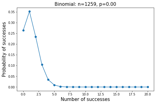
Binomial distribution
Binomial probability density function
f(k)=\begin{pmatrix}n\\ k\\ \end{pmatrix} p^k(1-p)^{n-k} for\,\,k \,\,in \,\,\,{0,1,..., n}, 0\le p\le 1In probability theory and statistics, binomial distribution is a discrete probability distribution of the number of successes in n independent success / failure tests, in which the success probability of each test is p. Such a single success / failure test is also called Bernoulli test.
PMF (probability quality function) defines discrete random variable as the probability of discrete random variable in each specific value. Generally speaking, this function is used to calculate the probability of each successful event result for a discrete probability event.
Pdf (probability density function) is the definition of continuous random variable. Different from PMF, the value at a specific point is not the probability of that point. Continuous random probability events can only calculate the probability of events in a continuous area. By integrating this interval, the probability that the event occurrence time falls within a given interval can be obtained
from scipy.stats import binom
n = len(df['Returns'])
p = df['Returns'].mean()
k = np.arange(0,21)
Probability mass function
pmf(k,n,p,loc=0)
# Binomial distribution
binomial = binom.pmf(k,n,p)
plt.plot(k, binomial, 'o-')
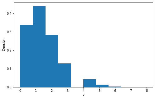
Function simulation binomial random variable
rvs(n, p, loc=0, size=1, random_state=None)
Use the rvs function to simulate a binomial random variable, where the parameter size specifies the number of times you want to simulate.
binom_sim = binom.rvs(n = n, p = p, size=10000)
print("Mean: %f" % np.mean(binom_sim))
print("SD: %f" % np.std(binom_sim, ddof=1))
plt.hist(binom_sim, bins = 10, density = True)
Mean: 1.323600 SD: 1.170991
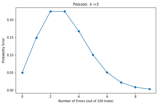
Poisson distribution
Parameters of Poisson distribution
\muIs the average number of random events per unit time (or unit area). Poisson distribution is suitable to describe the number of random events in unit time.
The expectation and variance of Poisson distribution are
\muPoisson distribution probability density function
f(k)=\exp(-\mu)\frac{\mu^k}{k!} k >0Probability mass function
rate = 3 # error rate
n = np.arange(0,10) # Number of experiments
y = stats.poisson.pmf(n, rate)
# pmf(k, mu, loc=0)
plt.plot(n, y, 'o-')
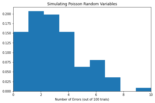
Simulated Poisson random variable
data = stats.poisson.rvs(mu=3, loc=0, size=100)
#  rvs(mu, loc=0, size=1, random_state=None)
print("Mean: %f" % np.mean(data))
print("Standard Deviation: %f" % np.std(data, ddof=1))
plt.hist(data, bins = 9, density = True, stacked=True)
Mean: 3.210000 Standard Deviation: 1.854805
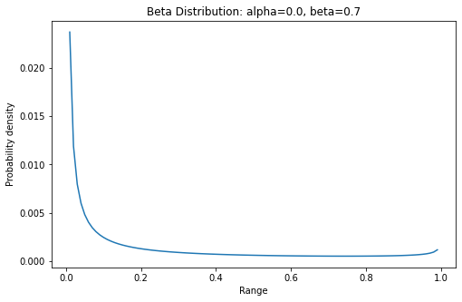
Beta distribution
Beta distribution is a density function as a conjugate prior distribution of Bernoulli distribution and binomial distribution. It has important applications in machine learning and mathematical statistics.
Beta distribution is a set defined in
(0,1)Continuous probability distribution of interval.
The probability density function of beta distribution is
f(x,a,b)=\frac{\Gamma(a+b)x^{a-1}(1-x)^{b-1}}{\Gamma(a)\Gamma(b)} 0<=x<=1,a>0,b>0\Gamma(z)=\int_0^\infty {t^{z-1}e^{-t}} \,{\rm d}tprobability density function
pdf(x, a, b, loc=0, scale=1)
x = np.arange(0, 1, 0.01)
y = stats.beta.pdf(x, alpha, beta)
plt.plot(x, y)
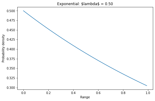
exponential distribution
Exponential distribution, also known as negative exponential distribution, is a probability distribution describing the time between events in Poisson process, that is, the process in which events occur continuously and independently at a constant average rate.
Its probability density function
f(X) = \begin{cases} \lambda e^{-\lambda x} & {x >0} \\[4ex] 0 & {x\le 0} \end{cases}lambd = 0.5 # lambda x = np.arange(0, 1, 0.01) y = lambd * np.exp(-lambd * x) plt.plot(x, y)
Lognormal distribution
Means that the logarithm of a random variable obeys the normal distribution, then the random variable obeys the lognormal distribution. Lognormal distribution is very close to normal distribution in the short term.
Probability density function of lognormal distribution
f(x,s)=\frac{1}{s x\sqrt{2 \pi} \exp \left(\frac{\log^2(x)}{2s^2}\right)} for \, x>0, s>0from scipy.stats import lognorm # mean value mu = df['Returns'].mean() #range sigma = df['Returns'].std()*math.sqrt(252) s = np.random.lognormal(mu, sigma, 1000) count, bins, ignored = plt.hist(s, 100, density=True, align='mid') x = np.linspace(min(bins), max(bins), 10000) pdf = (np.exp(-(np.log(x) - mu)**2 / (2 * sigma**2)) / (x * sigma * np.sqrt(2 * np.pi))) # pdf=lognorm.pdf(x, s, loc=0, scale=1) plt.plot(x, pdf, linewidth=2, color='r')
Calculate quantile
Quantile, also known as quantile, refers to the numerical points that divide the probability distribution range of a random variable into several equal parts. Commonly used are median (i.e. binary), quartile, percentile, etc.
# Calculate the quantiles of 5%, 25%, 75% and 95% of stock returns
# 5% quantile
>>> print('5% quantile', norm.ppf(0.05, mu, sigma))
'5% quantile  -0.548815100072449'
# 75% quantile
>>> print('75% quantile', norm.ppf(0.75, mu, sigma) )
'75% quantile  0.2265390517243559
Statistical hypothesis test
Hypothesis
General definition: a statement of an unknown fact. It will rain tomorrow
Extended to statistics, what are the "unknown facts" we are concerned about?
Statistical definition: a statement of the value of a population parameter. The overall parameters, including overall mean, proportion and variance, shall be stated before analysis. For example, suppose the average score of the final statistics exam is equal to 90 points.
Hypothesis testing
Definition: make some assumptions about the overall parameters or distribution form in advance, and then use the sample information to judge whether the original assumption is true.
Status: it is one of the two major methods of inferential statistics (parameter estimation and hypothesis test) in statistical methods (descriptive statistics and inferential statistics).
Application: commonly used in product production, product quality inspection and other issues.
In the hypothesis test, first set the original hypothesis (H0), and then set the opposite alternative hypothesis (H1). Next, samples are randomly selected. If the probability of sample occurrence (P) is very small when the original hypothesis is true, it indicates that the original hypothesis is not true, and the alternative hypothesis is true, the original hypothesis is rejected. Otherwise, accept the original hypothesis.
Process of hypothesis testing
(1) Make assumptions (2) Determine the appropriate test statistics (3) Specified significance level (4) Calculate the value of the test statistic (5) Make statistical decisions
Alpha: The significance level is the probability that the estimated population parameters may make mistakes when they fall within a certain interval. Is the probability of rejecting H0 when H0 is true. p-value: A probability, a probability of observed samples and more extreme cases on the premise that the original hypothesis is true. Reject the minimum significance level of the original hypothesis. P-value < = Alpha: reject H0. P-value > alpha: accept H0.
Specified significance level
Develop decision criteria. Calculate the confidence interval of z distribution.
alpha = 0.05
zleft = norm.ppf(alpha/2, 0, 1)
zright = -zleft  # The z distribution is symmetric
print(zleft, zright)
-1.9599639845400545 1.9599639845400545
Calculate the value of the statistic
mu = df['Returns'].mean()
sigma = df['Returns'].std(ddof=1)
n = df['Returns'].shape[0]
# If the sample size n is large enough, we can use z distribution instead of t distribution
# When H0 is true, mu = 0
zhat = (mu - 0)/(sigma/n**0.5)
print(zhat)
1.7823176948718935
Make statistical decisions
Decide whether to reject the original hypothesis.
print('The significant level is{},Do we refuse H0: {}
      '.format(alpha, zhat>zright or zhat<zleft))
The significance level was 0.05,Do we refuse H0: False
Unilateral test
mu = df['Returns'].mean()
sigma = df['Returns'].std(ddof=1)
n = df['Returns'].shape[0]
Determine the appropriate test statistics. If the sample size n is large enough, we can use z distribution instead of t distribution.
zhat = (mu - 0)/(sigma/n**0.5)
print(zhat)
1.7823176948718935
Specify the level of significance.
alpha = 0.05
zright = norm.ppf(1-alpha, 0, 1)
print(zright)
print('The significance level was{},Do we refuse H0: {}
      '.format(alpha, zhat>zright))
1.6448536269514722
 The significance level was 0.05,Do we refuse H0: True
p-value test
p_value = 1 - norm.cdf(zhat, 0, 1)
print(p_value)
print('The significance level was{},Do we refuse H0: {}
      '.format(alpha, p_value < alpha))
0.03734871936756168
 The significance level was 0.05,Do we refuse H0: True
scipy. Hypothesis testing in stats
Financial stock data is continuous data. For stock data, hypothesis testing is about comparing characteristics and targets or two samples. For some hypothesis tests, we can test a sample.
Continuous statistical distribution list [2]
Shapiro Wilk test
Shapiro Wilk test is used to verify whether a random sample data comes from normal distribution.
from scipy.stats import shapiro
import scipy as sp
W_test, p_value = shapiro(df['Returns'])
# The confidence level is 95%, i.e. alpha=0.05
print('Shapiro-Wilk Test')
print('-'*40)
# Significance decision
alpha = 0.05
if p_value < alpha:
    print("H0: The sample obeys Gaussian distribution")
    print("refuse H0")
else:
    print("H1: The sample does not obey Gaussian distribution")
    print("accept H0")
Shapiro-Wilk Test
----------------------------------------
H0: The sample obeys Gaussian distribution
 refuse H0
Anderson darling test
Whether the sample data of D'Agostino's K^2 Test comes from a specific distribution, including distribution: 'norm', 'expon', 'Gumbel', 'extreme 1' or 'logistic'
Null hypothesis H0: the sample follows a specific distribution; Alternative hypothesis H1: the sample does not obey a specific distribution
from scipy.stats import anderson
result = anderson(df['Returns'].dropna())
result
AndersonResult(
statistic=6.416543385168325,
critical_values=array([0.574, 0.654, 0.785, 0.915, 1.089]),
significance_level=array([15. , 10. ,  5. ,  2.5,  1. ]))
Make decisions
D'Agostino's K^2 Test
----------------------------------------
statistic: 6.417
15.000: 0.574, The sample does not obey the normal distribution (refuse H0)
10.000: 0.654, The sample does not obey the normal distribution (refuse H0)
5.000: 0.785, The sample does not obey the normal distribution (refuse H0)
2.500: 0.915, The sample does not obey the normal distribution (refuse H0)
1.000: 1.089, The sample does not obey the normal distribution (refuse H0)
Correlation is used to test whether samples or features are related. Therefore, check whether the two samples or features are related.
F-test
F-test, the most commonly used alias, is called joint hypothesis test. It is a test that the statistical value obeys the F-distribution under the null hypothesis (H0).
import scipy
from scipy.stats import f

F = df['Adj Close'].var() / df['Returns'].var()
df1 = len(df['Adj Close']) - 1
df2 = len(df['Returns']) - 1
p_value = scipy.stats.f.cdf(F, df1, df2)
Make decisions
F-test
----------------------------------------
Statistic: 1.000
H0: The samples are independent of each other. p=1.000
Pearson correlation coefficient
Pearson's Correlation Coefficient, also known as product moment correlation (or product moment correlation), is a method for calculating linear correlation proposed by British statistician Pearson in the 20th century.
Scope of application
The correlation coefficient is defined only when the standard deviation of both variables is not zero. Pearson correlation coefficient is applicable to:
(1) There is a linear relationship between the two variables, which are continuous data. (2) The population of the two variables is normal distribution, or near normal unimodal distribution. (3) The observations of the two variables are paired, and each pair of observations is independent of each other.
from scipy.stats import pearsonr
coef, p_value = pearsonr(df['Open'],
                    df['Adj Close'])
Make decisions
Pearson correlation coefficient
----------------------------------------
Correlation test: 0.999
H1: There is correlation between samples. p=0.000
Spearman rank correlation
Spearman rank correlation is a method to study the correlation between two variables according to rank data. It is calculated according to the difference between the number of pairs of grades in two columns, so it is also called "grade difference method".
Spearman rank correlation has no strict requirements on data conditions. As long as the observed values of two variables are paired grade evaluation data or grade data transformed from continuous variable observation data, Spearman rank correlation can be used for research regardless of the overall distribution form and sample capacity of the two variables.
Spearman's rank correlation coefficient reflects the closeness of the relationship between the two groups of variables. It is the same as the correlation coefficient r, with a value range of [- 1, + 1], except that it is calculated on the basis of rank.
from scipy.stats import spearmanr
coef, p_value = spearmanr(df['Open'], df['Adj Close'])
Make decisions
Spearman rank correlation
----------------------------------------
Spearman rank correlation coefficient: 0.997
 There is correlation between samples (refuse H0) p=0.000
Kendall Correlation
Kendall's rank correlation coefficient is a statistical value used to measure the correlation between two random variables. A Kendall test is a nonparametric hypothesis test, which uses the calculated correlation coefficient to test the statistical dependence of two random variables.
The Kendall correlation coefficient ranges from - 1 to 1
- When τ When it is 1, it means that the two random variables have consistent rank correlation;
- When τ When it is - 1, it means that the two random variables have completely opposite rank correlation;
- When τ When it is 0, it means that the two random variables are independent of each other.
from scipy.stats import kendalltau
coef, p_value = kendalltau(df['Open'],
                  df['Adj Close'])
Make decisions
Kendall Correlation
----------------------------------------
Kendall rank correlation coefficient: 0.960
 There is correlation between samples (refuse H0) p=0.000
Chi square test
Chi square test is a widely used hypothesis test method. Its application in statistical inference of classified data includes: Chi square test for comparison of two rates or two constituent ratios; Chi square test for comparison of multiple rates or multiple constituent ratios and correlation analysis of classified data.
In big data operation scenarios, it is usually used to determine whether the value of a variable (or characteristic) is significantly related to the dependent variable.
from scipy.stats import chi2_contingency
from scipy.stats import chi2
stat, p_value, dof, expected = chi2_contingency(df[['Open','Low','High','Adj Close','Volume']])
prob = 0.95
critical = chi2.ppf(prob, dof)
Statistical decision
abs(stat) >= critical
dof=5032
 possibility=0.950,
critical=5198.140, stat=259227.557
 The two are related (refuse H0)
p-valued decision
p <= alpha
Significance=0.050, p=0.000
 The two are related (refuse H0)
This part is to compare two samples or characteristics; Get the results and check whether they are independent samples.
scipy. Other hypothesis tests in stats
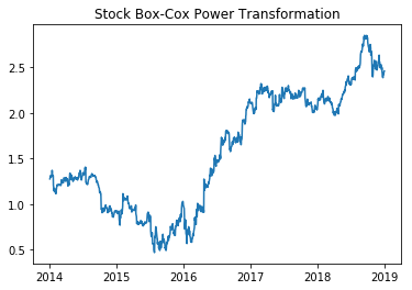
Box-Cox Power Transformation
Box cox Transformation can convert independent dependent variables with non normal distribution into normal distribution. We know that an important assumption of many statistical test methods is "normality". Therefore, after Box cox Transformation, it means that we can carry out many kinds of statistical tests on our data.
The main feature of box Cox transform is to introduce a parameter, estimate the parameter through the data itself, and then determine the data transformation form that should be adopted. Box Cox transform can significantly improve the normality, symmetry and variance equality of data, and is effective for many practical data.
>>> from scipy.stats import boxcox
>>> df['boxcox'], lam = boxcox(df['Adj Close'])
>>> print('Lambda: %f' % lam)
Lambda: -0.119624
Line chart
plt.plot(df['boxcox'])
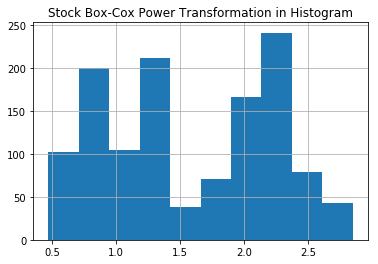
histogram
plt.hist(df['boxcox'])
The following hypothesis tests are only simple and do not give too many other explanations.
# Parametric hypothesis test
# Student's t-Test
# This is a two-sided test of the original hypothesis. Two independent samples have the same
# Average (expected value) of.
# This test assumes that the population has the same variance by default.
from scipy.stats import ttest_ind
stat, p_value = ttest_ind(df['Open'],
    df['Adj Close'])

# Paired Student's t-test
# This is a two-sided test of the original hypothesis,
# That is, two related or repeated samples have the same average (expected value)
from scipy.stats import ttest_rel
stat, p_value = ttest_rel(df['Open'],
    df['Adj Close'])

# Analysis of Variance Test (ANOVA)
from scipy.stats import f_oneway
stat, p_value = f_oneway(df['Open'],
    df['Adj Close'], df['Volume'])

# Nonparametric hypothesis test
# Mann-Whitney U Test
from scipy.stats import mannwhitneyu
stat, p_value = mannwhitneyu(df['Open'],
    df['Adj Close'])

# Wilcoxon Signed-Rank Test
from scipy.stats import wilcoxon
stat, p_value = wilcoxon(df['Open'],
    df['Adj Close'])

# Kruskal-Wallis Test
from scipy.stats import kruskal
stat, p_value = kruskal(df['Open'],
    df['Adj Close'], df['Volume'])

# Levene Test
from scipy.stats import levene
stat, p_value = levene(df['Open'],
    df['Adj Close'])

# Mood's Test
from scipy.stats import mood
stat, p_value = mood(df['Open'],
    df['Adj Close'])

# Mood's median test
from scipy.stats import median_test
stat, p_value, med, tbl = median_test(df[
  'Open'], df['Adj Close'], df['Volume'])

# Kolmogorov-Smirnov test
from scipy.stats import ks_2samp
stat, p_value = ks_2samp(df['Open'],
    df['Adj Close'])
reference material
[1]
Common stock probability distribution methods: https://www.investopedia.com/articles/06/probabilitydistribution.asp
[2]
Continuous statistical distribution list: https://docs.scipy.org/doc/scipy/reference/tutorial/stats/continuous.html