The previous article explained the logistic regression model of deep learning. This article will next talk about the vectorization of logistic regression and the basic code required for compilation.

 

1.sigmoid function:

                                                     

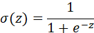
The sigmoid function can be compiled using python's math libraryHowever, such compilation cannot be applied to a huge matrix database (using a matrix as a variable will report an error)

import math
def basic_sigmoid(x):
    s = 1 / (1 + math.exp(-x))
    return s
basic_sigmoid([1,2,3])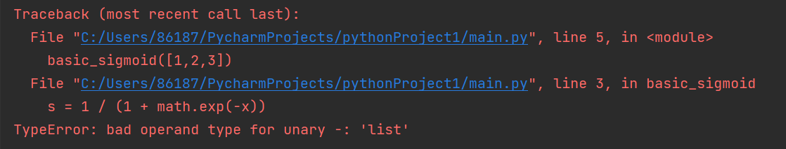

Here we refer to the numpy library to operate on the matrix

import numpy as np
x = np.array([1, 2, 3])
print(np.exp(x))

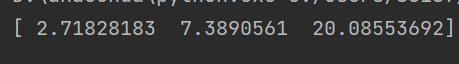
In this way, we will not report an error, so we successfully apply the sigmoid function to the matrix

The introduction of numpy library is placed below, and readers can view it by themselves

(18 messages) introduction to Python numpy Library_ A little white who writes a blog silently - CSDN bloghttps://blog.csdn.net/qq_41644183/article/details/88732405?ops_request_misc=%257B%2522request%255Fid%2522%253A%2522163470996316780357231248%2522%252C%2522scm%2522%253A%252220140713.130102334..%2522%257D&request_id=163470996316780357231248&biz_id=0&utm_medium=distribute.pc_search_result.none-task-blog-2~all~sobaiduend~default-2-88732405.pc_search_result_hbase_insert&utm_term=python+numpy%E5%BA%93%E7%AE%80%E4%BB%8B&spm=1018.2226.3001.4187

Therefore, we use numpy function library to convert the input data into a matrix through np.array, or use np.reshape to change the dimension of the matrix, which can easily convert the data into a one-dimensional matrix we want.

For example, when recognizing a picture, put the rgb pixel value of the tee sleeve of the picture into a feature vector:

Let's take a look at how a picture is represented in the computer. In order to save a picture, you need to save three matrices, which correspond to the red, green and blue color channels in the picture. If your picture is 64x64 pixels in size, you have three 64x64 matrices, which correspond to the intensity values of the red, green and blue pixels in the picture. By inputting three channel pixel values, i.e. three matrices of 64x64, we can use the np.reshape function to put them into a matrix:

import numpy as np
def image2vector(image):
    v = image.reshape((image.shape[0] * image.shape[1] * image.shape[2], 1))
    return v
image = np.array([[[ 0.67826139,  0.29380381],
        [ 0.90714982,  0.52835647],
        [ 0.4215251 ,  0.45017551]],

       [[ 0.92814219,  0.96677647],
        [ 0.85304703,  0.52351845],
        [ 0.19981397,  0.27417313]],

       [[ 0.60659855,  0.00533165],
        [ 0.10820313,  0.49978937],
        [ 0.34144279,  0.94630077]]])
print(image2vector(image))

The operation effect is shown in the figure, and the 3x2 three-dimensional matrix is successfully converted to 18x1 one-dimensional matrix

A very important concept to understand in numpy is "broadcasting". It is very useful for mathematical operations between arrays of different shapes.

Let's take an example:

import numpy as np
def softmax(x):
    x_exp = np.exp(x)    #Use the sigmoid function for all elements
    x_sum = np.sum(x_exp, axis=1, keepdims=True)   #Accumulate rows
    s = x_exp / x_sum        #Each element is divided by the sum of the corresponding row
    return s

x = np.array([
    [9, 2, 5, 0, 0],
    [7, 5, 0, 0 ,0]])
print("softmax(x) = " + str(softmax(x)))

Where np.sum (x, axis = 0 × 1, keepdims = true)

When axis=1, the matrix is added by columns, that is, the sum of columns is calculated

When axis=2, the matrix is added by rows, that is, the sum of rows

keepdims is used to maintain the dimension property of the matrix (children's shoes that don't understand can find the function by themselves)

The output results are as follows

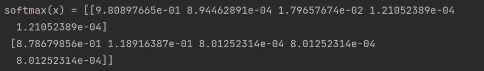
  This is how to calculate the proportion of two lines after sigmoid function operation

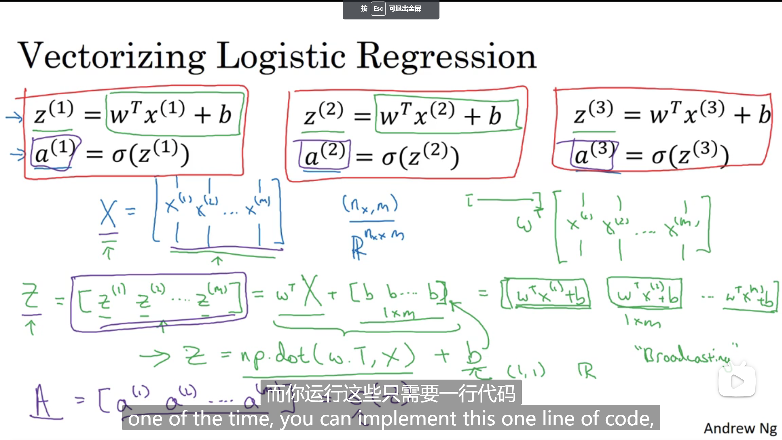
Vectorization:

In deep learning, if for loop and while loop are used to traverse each data, the algorithm will become inefficient. At the same time, there will be more and more large data sets in the field of deep learning, so it will be important to apply your algorithm without explicit for loop, and it will help you apply to larger data sets. The function of vectorization is to reduce operation time and optimize algorithm

import time #Import time library
a = np.random.rand(1000000)
b = np.random.rand(1000000) #Two arrays with one million dimensions are randomly obtained through round
tic = time.time() #Now measure the current time
#Vectorized version
c = np.dot(a,b)
toc = time.time()
print('Vectorized version:' + str(1000*(toc-tic)) +'ms') #Print the time of the vectorized version

#Continue to add non vectorized versions
c = 0
tic = time.time()
for i in range(1000000):
    c += a[i]*b[i]
toc = time.time()
print(c)
print('For loop:' + str(1000*(toc-tic)) + 'ms')#Time to print the version of the for loop

The return value is shown in the figure

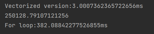
It can be seen that the operation time is almost 100 times faster

Similarly, by using vectorization, we can reduce the amount of computation of (matrix transpose) wt * X (eigenvector)

In the previous article, we talked about the need for cyclic gradient descent after finding the partial derivative. If w is a vector above two dimensions, we need to gradient descent w1, w2, etc. but if we define DW as a matrix and put dw1, dw2, etc. into the matrix for operation again and again, we can reduce for traversal, so as to improve the performance of the algorithm

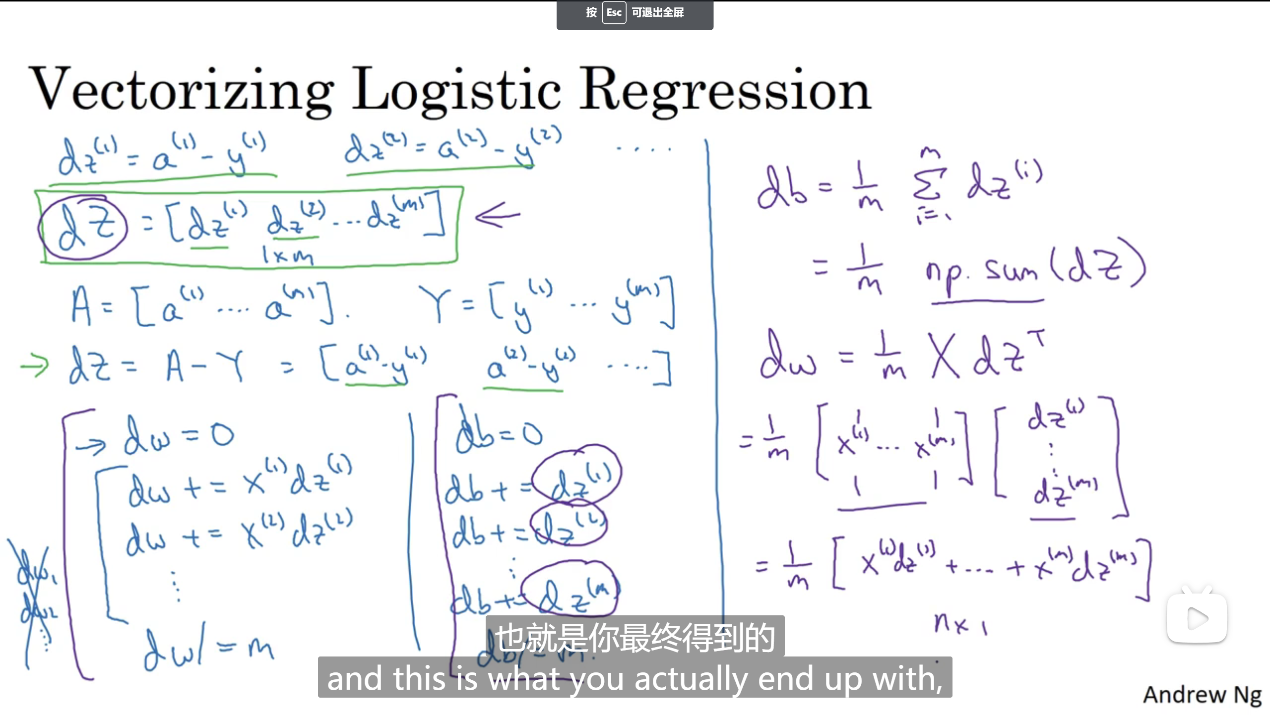
Data sets are the same. Put them into the matrix and use point multiplication to calculate