Python wechat ordering applet course video
https://edu.csdn.net/course/detail/36074
Python actual combat quantitative transaction financial management system
https://edu.csdn.net/course/detail/35475 catalogue
- Technical background
- Simulation of air resistance
- Impact of adding arc coil
- Chopping arc
- Summary summary
- Copyright notice
Back to the top #Technical background
As a national ball, table tennis has not only received many medals for China in many stadiums such as the Olympic Games, but also is widely liked by everyone in the people. stay Last blog It mainly describes the application of Magnus force in the movement of table tennis, and can see the arc track under various rotations of table tennis from the perspective of top view. This paper mainly describes the influence of air resistance on the movement process of table tennis.
Back to the top #Simulation of air resistance
The expression of air resistance we know is:
F=CρSv2F=C\rho Sv^2
Where C is a constant, which may be different for different material parameters. This needs to be measured in the experiment, and here we can simply take a hypothetical value. ρ\ rho is the air density, S is the windward area. For a table tennis ball, the windward area is actually the projected area of the table tennis ball, v is the speed, and the air resistance is directly proportional to the square of the speed. As for the direction of resistance, it is the opposite direction of resistance. Relevant simulation test codes are as follows:
1
2
3
4
5
6
7
8
9
10
11
12
13
14
15
16
17
18
19
20
21
22
23
24
25
26
27
28
29
30
31
32
33
34
35
36
37
38
39
40
41
import numpy as np
from tqdm import trange
import matplotlib.pyplot as plt

vel = np.array([4.,4.])
vel0 = vel.copy()
steps = 100
r = 0.02
rho = 1.29
mass_min = 2.53e-03
mass_max = 2.70e-03
dt = 0.01
g = 9.8
C = 0.1
s0 = np.array([0.,0.])
s00 = np.array([0.,0.])

s1 = [s0.copy()]
for step in trange(steps):
    s0 += vel*dt
    s1.append(s0.copy())
    # print (vel)
    vel += np.array([0.,-g])*dt
s1 = np.array(s1)

s2 = [s00.copy()]
for step in trange(steps):
    s00 += vel0*dt
    s2.append(s00.copy())
    vel_norm = np.linalg.norm(vel0)
    DampF = C*rho*np.pi*r**2*vel_norm**2
    DampA = DampF/mass_min
    # print (vel)
    vel0 -= np.array([DampA*vel0[0]/vel_norm, DampA*vel0[1]/vel_norm])*dt
    vel0 += np.array([0.,-g])*dt
s2 = np.array(s2)

plt.figure()
plt.plot(s1[:,0], s1[:,1], 'o', color='orange')
plt.plot(s2[:,0], s2[:,1], 'o', color='black')
plt.savefig('damping.png')
The running results of the code are shown in the figure below. The orange track represents the curve without added resistance, and the black track represents the air resistance considered:
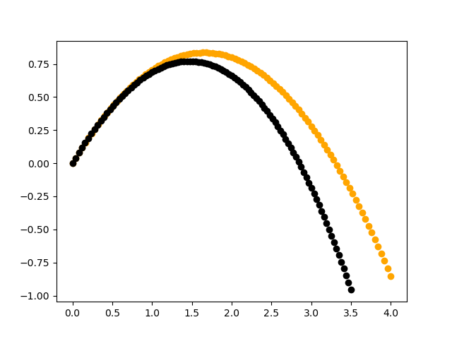
It can be seen that after adding air resistance, the speed of table tennis gradually decreases, and it is no longer a beautiful parabola. It should be noted that our trajectory here is a side view viewed from the y-z plane.
Back to the top #Impact of adding arc coil
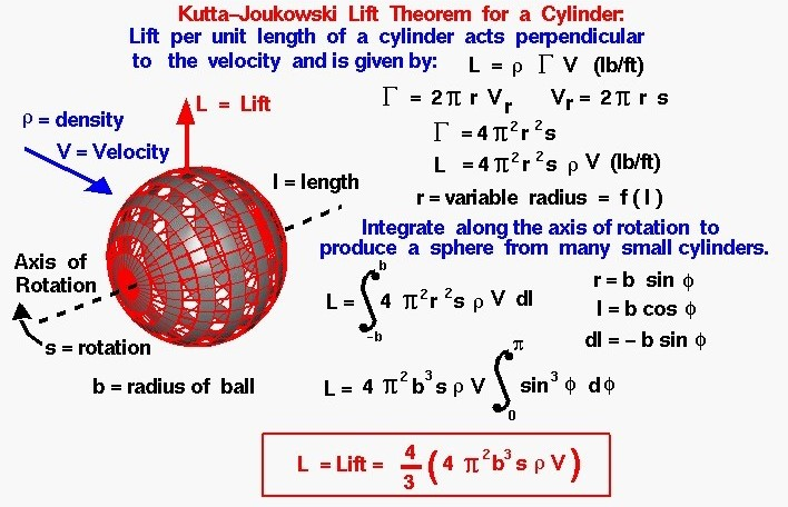
In the last chapter, we mainly considered the influence of air resistance on the trajectory of table tennis, which did not consider the rotation of table tennis itself. Here, we consider a scene of a circle ball: the trajectory of adding a rotating circle or a high hanging circle ball. The upward rotation needs to be added to the trajectory of the table tennis activity. The upward rotation will bring a downward Magnus force to the table tennis, making the arc of the table tennis trajectory smaller. The specific form of Magnus force refers to the Kutta JOUKOWSKI theory provided by Nasa as follows:
The relevant simulation codes are as follows. Here, in order to facilitate the call, we package the module generating the track into a simple function:
1
2
3
4
5
6
7
8
9
10
11
12
13
14
15
16
17
18
19
20
21
22
23
24
25
26
27
28
29
30
31
32
33
34
35
36
37
38
39
40
41
42
43
44
45
46
47
48
49
import numpy as np
from tqdm import trange
import matplotlib.pyplot as plt

vel = np.array([4.,4.])
vel0 = vel.copy()
steps = 100
r = 0.02
rho = 1.29
mass_min = 2.53e-03
mass_max = 2.70e-03
dt = 0.01
g = 9.8
C = 0.1
f0 = 0.
f1 = 0.
omega0 = 4
s0 = np.array([0.,0.])
s00 = np.array([0.,0.])

def F(vel, omega, r, rho):
    return 4*(4*np.pi**2*r**3*omega*vel*rho)/3

def Trace(steps, s0, vel0, f0, f1, dt, mass, omega0, r, rho, damping=False, KJ=False):
    s = [s0.copy()]
    tmps = s0.copy()
    for step in trange(steps):
        tmps += vel0*dt+0.5*f0*dt**2/mass
        s.append(tmps.copy())
        vel_norm = np.linalg.norm(vel0)
        if KJ:
            vel0 += np.array([np.sqrt(vel0[1]**2*(f0*dt/mass)**2/(vel0[0]**2+vel0[1]**2)),
                             -np.sqrt(vel0[0]**2*(f0*dt/mass)**2/(vel0[0]**2+vel0[1]**2))])
        if damping:
            vel0 -= np.array([f1*vel0[0]/vel_norm, f1*vel0[1]/vel_norm])*dt/mass
        vel0 += np.array([0.,-g])*dt
        f0 = F(np.linalg.norm(vel0), np.abs(omega0), r, rho)
        f1 = C*rho*np.pi*r**2*vel_norm**2
    return np.array(s)

s1 = Trace(steps, s0, vel0.copy(), f0, f1, dt, mass_min, omega0, r, rho, damping=False, KJ=False)
s2 = Trace(steps, s0, vel0.copy(), f0, f1, dt, mass_min, omega0, r, rho, damping=True, KJ=False)
s3 = Trace(steps, s0, vel0.copy(), f0, f1, dt, mass_min, omega0, r, rho, damping=True, KJ=True)

plt.figure()
plt.plot(s1[:,0], s1[:,1], 'o', color='orange')
plt.plot(s2[:,0], s2[:,1], 'o', color='black')
plt.plot(s3[:,0], s3[:,1], 'o', color='red')
plt.savefig('damping.png')
The operation results are as follows. The Yellow track indicates that the effect of air resistance and Magnus force is not considered, while the black track indicates that the effect of air resistance and Magnus force is not considered. The relevant contents have been introduced in the previous chapter. Finally, a red track indicates that the results of air resistance and Magnus force are considered at the same time, That is, the effect of normally pulled high hanging arc ball:
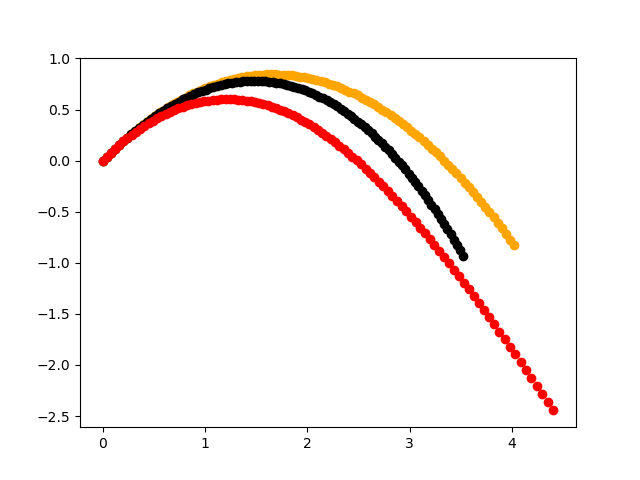
From this result, we can know that the high hanging arc ball not only rotates strongly, but also becomes more low and flat on the track, which is a strong threat on the field.
Back to the top #Chopping arc
In the last chapter, we simulated the result of high hanging loop ball, that is, the ball rotating upward, and there is another non loop playing method on the field: the combination of cutting and attacking. The chopping technology can bring a strong downward rotation to the ball, which changes the direction of mag's efforts. The relevant simulation codes are as follows:
1
2
3
4
5
6
7
8
9
10
11
12
13
14
15
16
17
18
19
20
21
22
23
24
25
26
27
28
29
30
31
32
33
34
35
36
37
38
39
40
41
42
43
44
45
46
47
48
49
50
51
52
import numpy as np
from tqdm import trange
import matplotlib.pyplot as plt

vel = np.array([4.,4.])
vel0 = vel.copy()
steps = 100
r = 0.02
rho = 1.29
mass_min = 2.53e-03
mass_max = 2.70e-03
dt = 0.01
g = 9.8
C = 0.1
f0 = 0.
f1 = 0.
omega0 = 4
s0 = np.array([0.,0.])
s00 = np.array([0.,0.])

def F(vel, omega, r, rho):
    return 4*(4*np.pi**2*r**3*omega*vel*rho)/3

def Trace(steps, s0, vel0, f0, f1, dt, mass, omega0, r, rho, damping=False, KJ=False, down\_spin=False):
    s = [s0.copy()]
    tmps = s0.copy()
    for step in trange(steps):
        tmps += vel0*dt+0.5*f0*dt**2/mass
        s.append(tmps.copy())
        vel_norm = np.linalg.norm(vel0)
        if KJ and not down_spin:
            vel0 += np.array([np.sqrt(vel0[1]**2*(f0*dt/mass)**2/(vel0[0]**2+vel0[1]**2)),
                              -np.sqrt(vel0[0]**2*(f0*dt/mass)**2/(vel0[0]**2+vel0[1]**2))])
        if KJ and down_spin:
            vel0 += np.array([-np.sqrt(vel0[1]**2*(f0*dt/mass)**2/(vel0[0]**2+vel0[1]**2)),
                              np.sqrt(vel0[0]**2*(f0*dt/mass)**2/(vel0[0]**2+vel0[1]**2))])
        if damping:
            vel0 -= np.array([f1*vel0[0]/vel_norm, f1*vel0[1]/vel_norm])*dt/mass
        vel0 += np.array([0.,-g])*dt
        f0 = F(np.linalg.norm(vel0), omega0, r, rho)
        f1 = C*rho*np.pi*r**2*vel_norm**2
    return np.array(s)

s1 = Trace(steps, s0, vel0.copy(), f0, f1, dt, mass_min, omega0, r, rho, damping=True, KJ=False)
s2 = Trace(steps, s0, vel0.copy(), f0, f1, dt, mass_min, omega0, r, rho, damping=True, KJ=True)
s3 = Trace(steps, s0, vel0.copy(), f0, f1, dt, mass_min, omega0, r, rho, damping=True, KJ=True, down_spin=True)

plt.figure()
plt.plot(s1[:,0], s1[:,1], 'o', color='orange')
plt.plot(s2[:,0], s2[:,1], 'o', color='black')
plt.plot(s3[:,0], s3[:,1], 'o', color='red')
plt.savefig('damping.png')
In this simulation, we compared the arc without arc (orange track), high hanging arc (black track) and chopping arc (red track), as shown in the following figure:
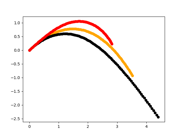
From the results, we find that the strong downward rotation brings the rising Magnus force to the table tennis, so the arc trajectory of the table tennis is elongated, which is relatively easier to control the arc. For example, Zhu Shihe, Matt of the Chinese team and Hou Yingying of the former national team are famous choppers.
Back to the top #Summary summary
In the previous blog, we introduced the simulation of table tennis arc technology with side rotation. In this paper, we focus on the two trajectory principles of high hanging arc and chopping arc, and introduce the influence of air resistance on the trajectory of table tennis. Through the simulation of air resistance and Magnus force, we can see different arc curves. For table tennis lovers, the results of this simulation can be used to formulate strategies that may be used in the game, such as low long circle ball, high short circle ball and so on. First formulate the strategy from a scientific perspective, then improve the technical level through daily training and consolidation, and finally use it in the formal competition.
Back to the top #Copyright notice
The first link of this article is: https://blog.csdn.net/dechinphy/p/damping.html
Author ID: DechinPhy
For more original articles, please refer to: https://blog.csdn.net/dechinphy/
Special links for rewards: https://blog.csdn.net/dechinphy/gallery/image/379634.html
Tencent cloud column synchronization: https://cloud.tencent.com/developer/column/91958