github address: DataScicence
Integrated learning 5-Xgboost principle and parameter tuning
Integrated learning 4-forward step-by-step algorithm and GBDT principle and case
Principles and cases of integrated learning 3-Boosting
Principle and case analysis of integrated learning 2-bagging
Principle and case analysis of integrated learning 1- voting method

Blending

principle

Steps:

• Divide data into trains_ data,Validate_data,Test_data three parts
• First layer model:
  • Using multiple base models in Train_data to get multiple models M k M^k Mk
  • Validate separately_ data,Test_ Data input model to get the prediction label A k , B k A^k,B^k Ak,Bk
• Layer 2 model:
  • Use prediction labels on validation sets A k A^k Ak is used as the input and the real label is used as the output. The model is trained on the meta model N N N
  • take B k B^k Bk is used as the input and N models are input to obtain the final prediction label on the test set T T T
• Evaluation model effect

Examples

import numpy as np 
import pandas as pd 
import matplotlib.pyplot as plt 
import seaborn as sns

Import data

from sklearn.datasets import load_iris

data = load_iris()

X = data.data[:,1:3]
y = data.target
print(X.shape,y.shape)

(150, 2) (150,)

Data division

from sklearn.model_selection import train_test_split

X_train_,X_test,y_train_,y_test = train_test_split(X,y,test_size = 0.2)

X_train,X_val,y_train,y_val = train_test_split(X_train_,y_train_)

print(X_train.shape,X_val.shape,X_test.shape)

(90, 2) (30, 2) (30, 2)

First layer classifier

from sklearn.svm import SVC
from sklearn.tree import DecisionTreeClassifier
from sklearn.neighbors import KNeighborsClassifier

# Model M^k
clfs = [SVC(probability = True),DecisionTreeClassifier(),KNeighborsClassifier()]

val_features = np.zeros((X_val.shape[0],len(clfs)))  # A^k
test_features = np.zeros((X_test.shape[0],len(clfs)))  #B^k

for i,clf in enumerate(clfs):
    clf.fit(X_train,y_train)
    val_feature = clf.predict_proba(X_val)[:, 1]
    test_feature = clf.predict_proba(X_test)[:,1]
    val_features[:,i] = val_feature
    test_features[:,i] = test_feature

Second layer classifier

from sklearn.linear_model import LogisticRegression
lr = LogisticRegression()

#Model N
lr.fit(val_features,y_val)
# Output predicted results
from sklearn.model_selection import cross_val_score
cross_val_score(lr,test_features,y_test,cv=5)

array([0.83333333, 0.66666667, 0.66666667, 0.83333333, 0.66666667])

Draw decision boundary

The Blending boundary here is not accurate, because the input of lr model is the prediction result of the first layer model, not the training data

from mlxtend.plotting import plot_decision_regions
import matplotlib.gridspec as gridspec
import itertools
clfs.append(lr)
gs = gridspec.GridSpec(2, 2)
fig = plt.figure(figsize=(10,8))
for clf, lab, grd in zip(clfs, 
                         ['SVC', 
                          'DT', 
                          'KNN',
                          'Blending'],
                          itertools.product([0, 1], repeat=2)):
    clf.fit(X, y)
    ax = plt.subplot(gs[grd[0], grd[1]])
    fig = plot_decision_regions(X=X, y=y, clf=clf)
    plt.title(lab)
plt.show()

stacking

principle

In Blending, our training model only uses part of the data, and the data is not fully utilized. Therefore, we can use cross validation to use all the data

Steps:

• Segment data into training set Train_data, test set_ data
• First layer model
  • K-fold cross validation is used on M models m respectively_ Data, and predict on K verification sets to get the prediction label A k ( take k individual junction fruit heap Fold ， And Discipline Practice number according to of long degree mutually with ) A ^ k (stack K results with the same length as the training data) AK (stack k results with the same length as the training data), predict on the test set and obtain the prediction label B k ( take K individual junction fruit plus power flat all ， And measure try collection long degree mutually with ) B ^ k (weighted average of K results, the same length as the test set) BK (weighted average of K results, the same length as the test set)
  • The results of m models are stacked vertically A m × k , B m × k A^{m\times k},B^{m\times k} Am×k,Bm×k
• Second layer model
  • use A m × k A^{m\times k} Am × k is used as input and trained on Meta model N to obtain model N
  • take B m × k B^{m\times k} Bm × k input model to get the final prediction result
• Evaluation model effect

Examples

from sklearn.model_selection import cross_val_score
from sklearn.linear_model import LogisticRegression
from sklearn.neighbors import KNeighborsClassifier
from sklearn.naive_bayes import GaussianNB 
from sklearn.ensemble import RandomForestClassifier
from mlxtend.classifier import StackingCVClassifier

model training

clf1 = KNeighborsClassifier(n_neighbors=1)
clf2 = RandomForestClassifier()
clf3 = GaussianNB()
lr = LogisticRegression()


clf_stacking = StackingCVClassifier(classifiers=[clf1,clf2,clf3],
                                   meta_classifier=lr,
                                   cv=5)
for clf, label in zip([clf1, clf2, clf3, clf_stacking], ['KNN', 'Random Forest', 'Naive Bayes','StackingClassifier']):
    scores = cross_val_score(clf, X, y, cv=3, scoring='accuracy')
    print("Accuracy: %0.2f (+/- %0.2f) [%s]" % (scores.mean(), scores.std(), label))

Accuracy: 0.91 (+/- 0.01) [KNN]
Accuracy: 0.95 (+/- 0.01) [Random Forest]
Accuracy: 0.91 (+/- 0.02) [Naive Bayes]
Accuracy: 0.96 (+/- 0.02) [StackingClassifier]

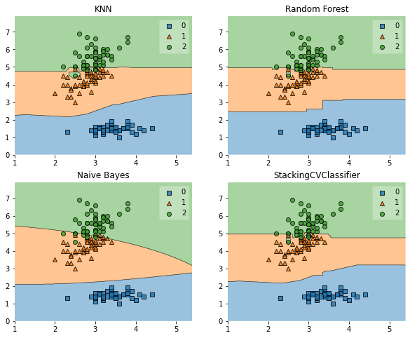
Decision boundary

from mlxtend.plotting import plot_decision_regions
from matplotlib import gridspec
import itertools

gs = gridspec.GridSpec(2,2)
fig =  plt.figure(figsize=(10,8))

for clf,lab,grd in zip([clf1,clf2,clf3,clf_stacking],
                      ['KNN', 
                          'Random Forest', 
                          'Naive Bayes',
                          'StackingCVClassifier'],
                       itertools.product([0,1],repeat=2)
                      ):
    clf.fit(X,y)
    ax = plt.subplot(gs[grd[0],grd[1]])
    fig = plot_decision_regions(X=X,y=y,clf=clf)
    plt.title(lab)
plt.show()

Grid parameter adjustment of stacking model

from sklearn.model_selection import GridSearchCV

params = {'kneighborsclassifier__n_neighbors': [1, 5],
          'randomforestclassifier__n_estimators': [10, 50],
          'meta_classifier__C': [0.1, 10.0]}

grid = GridSearchCV(estimator=clf_stacking, 
                    param_grid=params, 
                    cv=5,
                    refit=True)
grid.fit(X, y)
print('Best parameters: %s' % grid.best_params_)
print('Accuracy: %.2f' % grid.best_score_)

Best parameters: {'kneighborsclassifier__n_neighbors': 5, 'meta_classifier__C': 0.1, 'randomforestclassifier__n_estimators': 50}
Accuracy: 0.95

clf_stacking.score(X,y)

0.9866666666666667

The base model uses different feature subsets

from sklearn.pipeline import make_pipeline
from mlxtend.feature_selection import ColumnSelector
iris = load_iris()
X = iris.data
y = iris.target

pipe1 = make_pipeline(ColumnSelector(cols=(0, 2)),  # Select column 0,2
                      LogisticRegression())
pipe2 = make_pipeline(ColumnSelector(cols=(1, 2, 3)),  # Select columns 1, 2 and 3
                      LogisticRegression())

sclf = StackingCVClassifier(classifiers=[pipe1, pipe2], 
                            meta_classifier=LogisticRegression(),
                            random_state=42)

sclf.fit(X, y)

StackingCVClassifier(classifiers=[Pipeline(steps=[('columnselector',
                                                   ColumnSelector(cols=(0, 2))),
                                                  ('logisticregression',
                                                   LogisticRegression())]),
                                  Pipeline(steps=[('columnselector',
                                                   ColumnSelector(cols=(1, 2,
                                                                        3))),
                                                  ('logisticregression',
                                                   LogisticRegression())])],
                     meta_classifier=LogisticRegression(), random_state=42)

from sklearn.model_selection import cross_val_score
cross_val_score(sclf,X,y,cv=5)

array([0.96666667, 0.96666667, 0.9       , 0.96666667, 1.        ])