Background introduction

The basic principle of thermal power generation is: when the fuel is burned, it heats water to generate steam, the steam pressure drives the steam turbine to rotate, and then the steam turbine drives the generator to rotate to generate electric energy. In this series of energy conversion, the core affecting the power generation efficiency is the combustion efficiency of the boiler, that is, fuel combustion heats water to produce high-temperature and high-pressure steam. There are many factors affecting the combustion efficiency of the boiler, including the adjustable parameters of the boiler, such as combustion feed, primary and secondary air, induced air, return air and water supply; And the working conditions of the boiler, such as boiler bed temperature and bed pressure, furnace temperature and pressure, superheater temperature, etc. How can we use the above information to predict the amount of steam produced according to the working conditions of the boiler, so as to contribute to the output prediction of China's industrial industry?

Therefore, this case is to use the characteristics of the above industrial indicators to predict the steam volume. Due to information security and other reasons, we use the data collected by the desensitized boiler sensor (the acquisition frequency is minute level).

Data information

The data is divided into training data (train.txt) and test data (test.txt), in which the fields "V0" - "V37" are used as characteristic variables and "target" is used as target variables. We need to use the training data to train the model and predict the target variables of the test data.

evaluating indicator

The final evaluation index is the mean square error MSE, namely:
S c o r e = 1 n ∑ 1 n ( y i − y i ∗ ) 2 Score = \frac{1}{n} {\textstyle \sum_{1}^{n}} (y_i-y_i^*)^2 Score=n1​∑1n​(yi​−yi∗​)2

Import package

import warnings
warnings.filterwarnings("ignore")
import matplotlib.pyplot as plt
import seaborn as sns

# Model
import pandas as pd
import numpy as np
from scipy import stats
from sklearn.model_selection import train_test_split
from sklearn.model_selection import GridSearchCV, RepeatedKFold, cross_val_score,cross_val_predict,KFold
from sklearn.metrics import make_scorer,mean_squared_error
from sklearn.linear_model import LinearRegression, Lasso, Ridge, ElasticNet
from sklearn.svm import LinearSVR, SVR
from sklearn.neighbors import KNeighborsRegressor
from sklearn.ensemble import RandomForestRegressor, GradientBoostingRegressor,AdaBoostRegressor
from xgboost import XGBRegressor
from sklearn.preprocessing import PolynomialFeatures,MinMaxScaler,StandardScaler

Load data

data_train = pd.read_csv('train.txt',sep = '\t')
data_test = pd.read_csv('test.txt',sep = '\t')

#Merge training data and test data
data_train["oringin"]="train"
data_test["oringin"]="test"
data_all=pd.concat([data_train,data_test],axis=0,ignore_index=True)
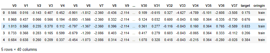
#Display the first 5 data
data_all.head()

Distribution exploration data

for column in data_all.columns[0:-2]:
    #Kernel density estimation is used to estimate the unknown density function in probability theory. It is one of the nonparametric test methods. Through the kernel density estimation diagram, we can intuitively see the distribution characteristics of the data samples themselves.
    g = sns.kdeplot(data_all[column][(data_all["oringin"] == "train")], color="Red", shade = True)
    g = sns.kdeplot(data_all[column][(data_all["oringin"] == "test")], ax =g, color="Blue", shade= True)
    g.set_xlabel(column)
    g.set_ylabel("Frequency")
    g = g.legend(["train","test"])
    plt.show()

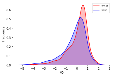
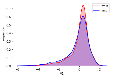
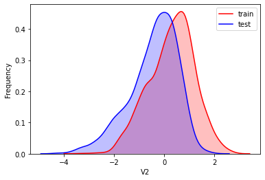
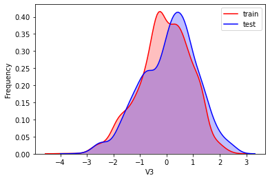
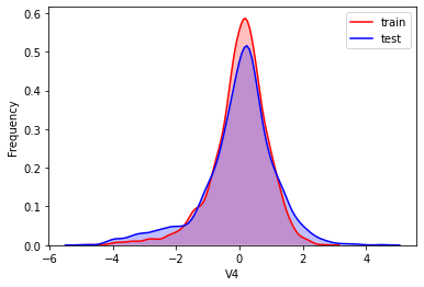
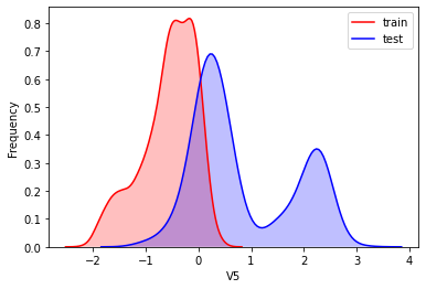
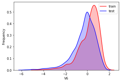
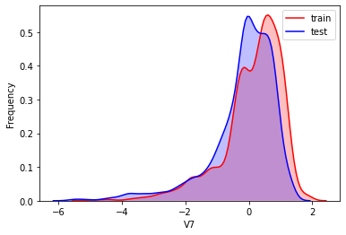
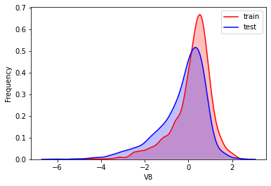
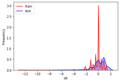
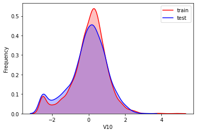
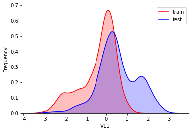
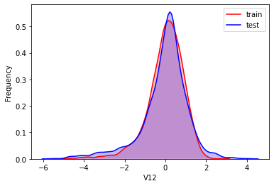
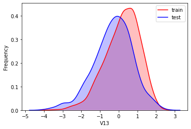
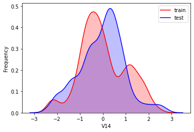
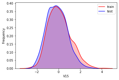
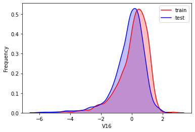
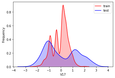
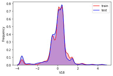
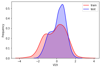
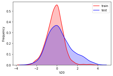
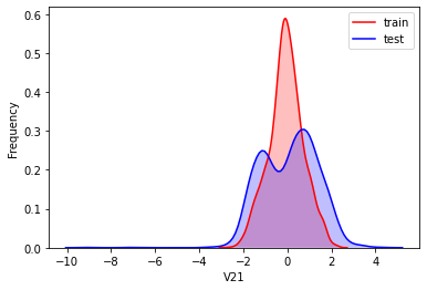
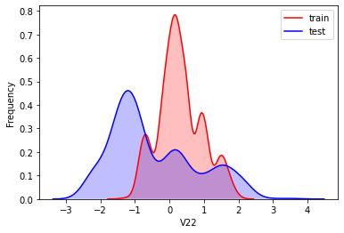
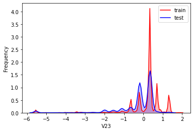
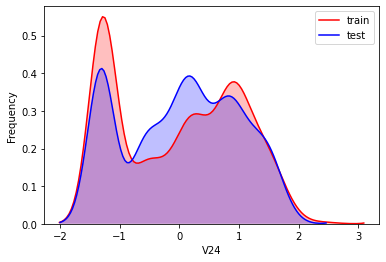
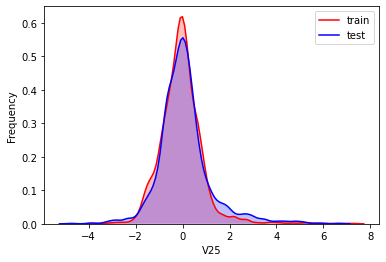
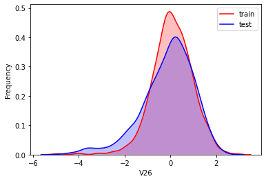
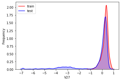
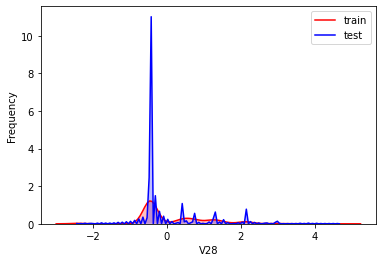
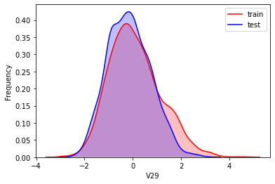
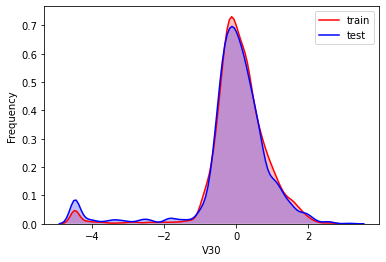
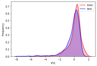
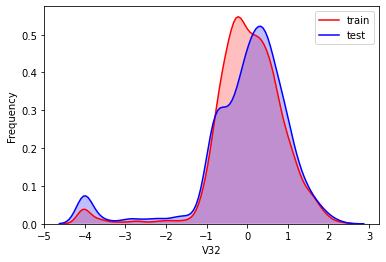
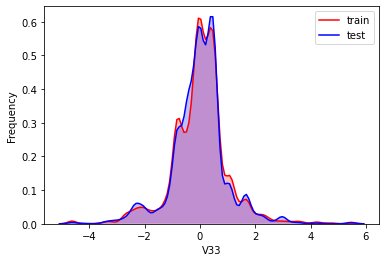
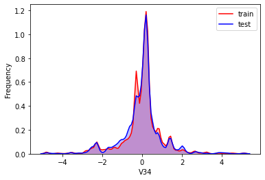
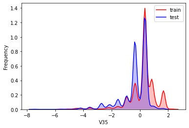
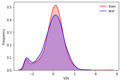
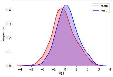
It can be seen from the above figure that the data distribution of training set and test set in features "V5", "V9", "V11", "V17", "V22" and "V28" is uneven, so we delete these feature data.

for column in ["V5","V9","V11","V17","V22","V28"]:
    g = sns.kdeplot(data_all[column][(data_all["oringin"] == "train")], color="Red", shade = True)
    g = sns.kdeplot(data_all[column][(data_all["oringin"] == "test")], ax =g, color="Blue", shade= True)
    g.set_xlabel(column)
    g.set_ylabel("Frequency")
    g = g.legend(["train","test"])
    plt.show()

data_all.drop(["V5","V9","V11","V17","V22","V28"],axis=1,inplace=True)

View the correlation between features (degree of correlation)

data_train1=data_all[data_all["oringin"]=="train"].drop("oringin",axis=1)
plt.figure(figsize=(20, 16))  # Specifies the width and height of the drawing object
colnm = data_train1.columns.tolist()  # List header
mcorr = data_train1[colnm].corr(method="spearman")  # The correlation coefficient matrix gives the correlation coefficient between any two variables
mask = np.zeros_like(mcorr, dtype=np.bool)  # It is constructed that the number matrix with the same dimension as mcorr is bool type
mask[np.triu_indices_from(mask)] = True  # True to the right of the corner divider
cmap = sns.diverging_palette(220, 10, as_cmap=True)  # Return matplotlib colormap object, color palette
g = sns.heatmap(mcorr, mask=mask, cmap=cmap, square=True, annot=True, fmt='0.2f')  # Thermodynamic diagram (see two similarity)
plt.show()

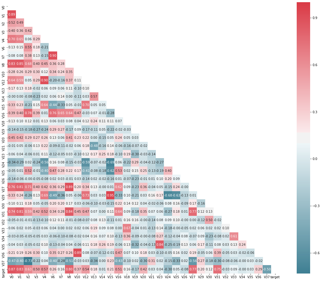
Dimensionality reduction operation, that is, delete the features whose absolute value of correlation is less than the threshold.

threshold = 0.1
corr_matrix = data_train1.corr().abs()
drop_col=corr_matrix[corr_matrix["target"]<threshold].index
data_all.drop(drop_col,axis=1,inplace=True)

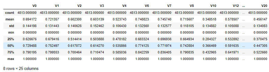
Normalize.

cols_numeric=list(data_all.columns)
cols_numeric.remove("oringin")
def scale_minmax(col):
    return (col-col.min())/(col.max()-col.min())
scale_cols = [col for col in cols_numeric if col!='target']
data_all[scale_cols] = data_all[scale_cols].apply(scale_minmax,axis=0)
data_all[scale_cols].describe()

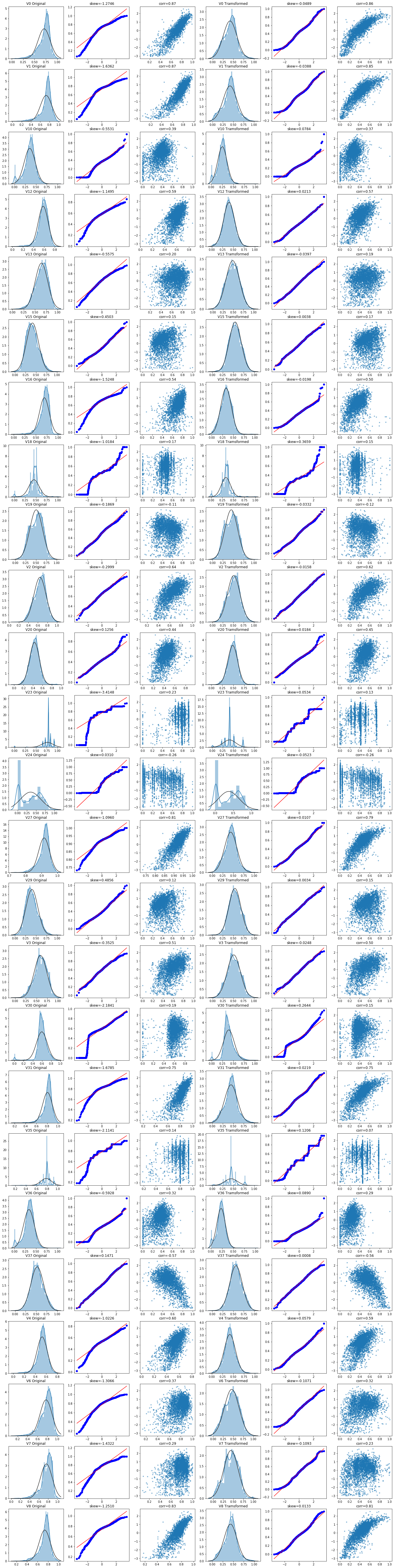
The plot shows the influence of box Cox transformation on data distribution. Box Cox is used when continuous response variables do not meet the normal distribution. After box Cox transform, the correlation between unobservable error and prediction variables can be reduced to a certain extent.

fcols = 6
frows = len(cols_numeric)-1
plt.figure(figsize=(4*fcols,4*frows))
i=0

for var in cols_numeric:
    if var!='target':
        dat = data_all[[var, 'target']].dropna()
        
        i+=1
        plt.subplot(frows,fcols,i)
        sns.distplot(dat[var] , fit=stats.norm);
        plt.title(var+' Original')
        plt.xlabel('')
        
        i+=1
        plt.subplot(frows,fcols,i)
        _=stats.probplot(dat[var], plot=plt)
        plt.title('skew='+'{:.4f}'.format(stats.skew(dat[var])))
        plt.xlabel('')
        plt.ylabel('')
        
        i+=1
        plt.subplot(frows,fcols,i)
        plt.plot(dat[var], dat['target'],'.',alpha=0.5)
        plt.title('corr='+'{:.2f}'.format(np.corrcoef(dat[var], dat['target'])[0][1]))
 
        i+=1
        plt.subplot(frows,fcols,i)
        trans_var, lambda_var = stats.boxcox(dat[var].dropna()+1)
        trans_var = scale_minmax(trans_var)      
        sns.distplot(trans_var , fit=stats.norm);
        plt.title(var+' Tramsformed')
        plt.xlabel('')
        
        i+=1
        plt.subplot(frows,fcols,i)
        _=stats.probplot(trans_var, plot=plt)
        plt.title('skew='+'{:.4f}'.format(stats.skew(trans_var)))
        plt.xlabel('')
        plt.ylabel('')
        
        i+=1
        plt.subplot(frows,fcols,i)
        plt.plot(trans_var, dat['target'],'.',alpha=0.5)
        plt.title('corr='+'{:.2f}'.format(np.corrcoef(trans_var,dat['target'])[0][1]))

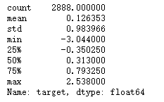
# Box Cox transformation
cols_transform=data_all.columns[0:-2]
for col in cols_transform:   
    # transform column
    data_all.loc[:,col], _ = stats.boxcox(data_all.loc[:,col]+1)
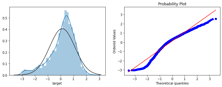
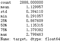
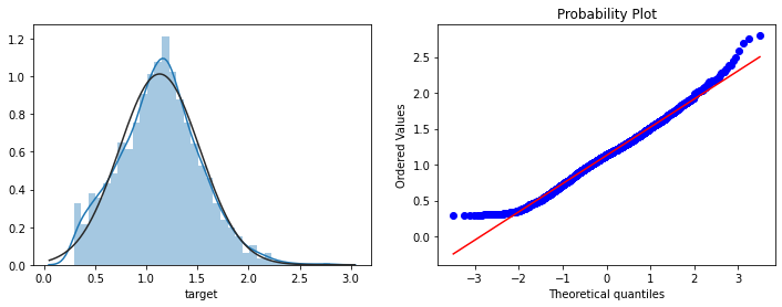
print(data_all.target.describe())
plt.figure(figsize=(12,4))
plt.subplot(1,2,1)
sns.distplot(data_all.target.dropna() , fit=stats.norm);
plt.subplot(1,2,2)
_=stats.probplot(data_all.target.dropna(), plot=plt)

Logarithmic transformation of target target value is used to improve the normality of characteristic data.

sp = data_train.target
data_train.target1 =np.power(1.5,sp)
print(data_train.target1.describe())

plt.figure(figsize=(12,4))
plt.subplot(1,2,1)
sns.distplot(data_train.target1.dropna(),fit=stats.norm);
plt.subplot(1,2,2)
_=stats.probplot(data_train.target1.dropna(), plot=plt)

Model building and integrated learning

Build training set and test set

# function to get training samples
def get_training_data():
    # extract training samples
    from sklearn.model_selection import train_test_split
    df_train = data_all[data_all["oringin"]=="train"]
    df_train["label"]=data_train.target1
    # split SalePrice and features
    y = df_train.target
    X = df_train.drop(["oringin","target","label"],axis=1)
    X_train,X_valid,y_train,y_valid=train_test_split(X,y,test_size=0.3,random_state=100)
    return X_train,X_valid,y_train,y_valid

# extract test data (without SalePrice)
def get_test_data():
    df_test = data_all[data_all["oringin"]=="test"].reset_index(drop=True)
    return df_test.drop(["oringin","target"],axis=1)

Evaluation function of rmse and mse

from sklearn.metrics import make_scorer
# metric for evaluation
def rmse(y_true, y_pred):
    diff = y_pred - y_true
    sum_sq = sum(diff**2)    
    n = len(y_pred)   
    return np.sqrt(sum_sq/n)

def mse(y_ture,y_pred):
    return mean_squared_error(y_ture,y_pred)

# scorer to be used in sklearn model fitting
rmse_scorer = make_scorer(rmse, greater_is_better=False) 

#Entered score_ When func is a scoring function, the value is True (default value); This value is False when the input function is a loss function
mse_scorer = make_scorer(mse, greater_is_better=False)

Find outliers and delete

# function to detect outliers based on the predictions of a model
def find_outliers(model, X, y, sigma=3):

    # predict y values using model
    model.fit(X,y)
    y_pred = pd.Series(model.predict(X), index=y.index)
        
    # calculate residuals between the model prediction and true y values
    resid = y - y_pred
    mean_resid = resid.mean()
    std_resid = resid.std()

    # calculate z statistic, define outliers to be where |z|>sigma
    z = (resid - mean_resid)/std_resid    
    outliers = z[abs(z)>sigma].index
    
    # print and plot the results
    print('R2=',model.score(X,y))
    print('rmse=',rmse(y, y_pred))
    print("mse=",mean_squared_error(y,y_pred))
    print('---------------------------------------')

    print('mean of residuals:',mean_resid)
    print('std of residuals:',std_resid)
    print('---------------------------------------')

    print(len(outliers),'outliers:')
    print(outliers.tolist())

    plt.figure(figsize=(15,5))
    ax_131 = plt.subplot(1,3,1)
    plt.plot(y,y_pred,'.')
    plt.plot(y.loc[outliers],y_pred.loc[outliers],'ro')
    plt.legend(['Accepted','Outlier'])
    plt.xlabel('y')
    plt.ylabel('y_pred');

    ax_132=plt.subplot(1,3,2)
    plt.plot(y,y-y_pred,'.')
    plt.plot(y.loc[outliers],y.loc[outliers]-y_pred.loc[outliers],'ro')
    plt.legend(['Accepted','Outlier'])
    plt.xlabel('y')
    plt.ylabel('y - y_pred');

    ax_133=plt.subplot(1,3,3)
    z.plot.hist(bins=50,ax=ax_133)
    z.loc[outliers].plot.hist(color='r',bins=50,ax=ax_133)
    plt.legend(['Accepted','Outlier'])
    plt.xlabel('z')
    
    return outliers

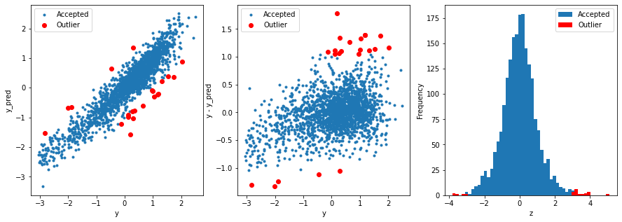
# get training data
X_train, X_valid,y_train,y_valid = get_training_data()
test=get_test_data()

# find and remove outliers using a Ridge model
outliers = find_outliers(Ridge(), X_train, y_train)
X_outliers=X_train.loc[outliers]
y_outliers=y_train.loc[outliers]
X_t=X_train.drop(outliers)
y_t=y_train.drop(outliers)

R2= 0.8766692300840107
rmse= 0.34900867702002514
mse= 0.12180705663526849

mean of residuals: -4.994630252296844e-16
std of residuals: 0.3490950546174426

22 outliers:
[2655, 2159, 1164, 2863, 1145, 2697, 2528, 2645, 691, 1085, 1874, 2647, 884, 2696, 2668, 1310, 1901, 1458, 2769, 2002, 2669, 1972]

Train the model

def get_trainning_data_omitoutliers():
    #Obtain training data and omit outliers
    y=y_t.copy()
    X=X_t.copy()
    return X,y

def train_model(model, param_grid=[], X=[], y=[], 
                splits=5, repeats=5):

    # get data
    if len(y)==0:
        X,y = get_trainning_data_omitoutliers()
        
    # Cross validation
    rkfold = RepeatedKFold(n_splits=splits, n_repeats=repeats)
    
    # Optimal parameters of grid search
    if len(param_grid)>0:
        gsearch = GridSearchCV(model, param_grid, cv=rkfold,
                               scoring="neg_mean_squared_error",
                               verbose=1, return_train_score=True)

        # train
        gsearch.fit(X,y)

        # Best model
        model = gsearch.best_estimator_        
        best_idx = gsearch.best_index_

        # Obtain cross validation evaluation indicators
        grid_results = pd.DataFrame(gsearch.cv_results_)
        cv_mean = abs(grid_results.loc[best_idx,'mean_test_score'])
        cv_std = grid_results.loc[best_idx,'std_test_score']

    # No grid search  
    else:
        grid_results = []
        cv_results = cross_val_score(model, X, y, scoring="neg_mean_squared_error", cv=rkfold)
        cv_mean = abs(np.mean(cv_results))
        cv_std = np.std(cv_results)
    
    # Merge data
    cv_score = pd.Series({'mean':cv_mean,'std':cv_std})

    # forecast
    y_pred = model.predict(X)
    
    # Statistics of model performance        
    print('----------------------')
    print(model)
    print('----------------------')
    print('score=',model.score(X,y))
    print('rmse=',rmse(y, y_pred))
    print('mse=',mse(y, y_pred))
    print('cross_val: mean=',cv_mean,', std=',cv_std)
    
    # Residual analysis and visualization
    y_pred = pd.Series(y_pred,index=y.index)
    resid = y - y_pred
    mean_resid = resid.mean()
    std_resid = resid.std()
    z = (resid - mean_resid)/std_resid    
    n_outliers = sum(abs(z)>3)
    outliers = z[abs(z)>3].index
    
    return model, cv_score, grid_results

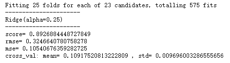
# Define training variables to store data
opt_models = dict()
score_models = pd.DataFrame(columns=['mean','std'])
splits=5
repeats=5

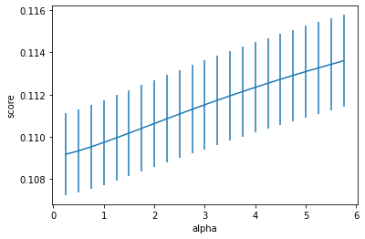
model = 'Ridge'  #Replaceable, see various models in case analysis I
opt_models[model] = Ridge() #Replaceable, see various models in case analysis I
alph_range = np.arange(0.25,6,0.25)
param_grid = {'alpha': alph_range}

opt_models[model],cv_score,grid_results = train_model(opt_models[model], param_grid=param_grid, 
                                              splits=splits, repeats=repeats)

cv_score.name = model
score_models = score_models.append(cv_score)

plt.figure()
plt.errorbar(alph_range, abs(grid_results['mean_test_score']),
             abs(grid_results['std_test_score'])/np.sqrt(splits*repeats))
plt.xlabel('alpha')
plt.ylabel('score')

1.LightGBM

import lightgbm as lgb

y_train = y_t.copy().values
X_train = X_t.copy().values
X_test =  get_test_data().values

#GBM decision tree
lgb_param = {
'num_leaves': 7, 
'min_data_in_leaf': 20, #The minimum number of records a leaf may have
'objective':'regression',
'max_depth': -1,
'learning_rate': 0.003,
"boosting": "gbdt", #Using gbdt algorithm
"feature_fraction": 0.18, #For example, 0.18 means that 18% of the parameters are randomly selected in each iteration to build the tree
"bagging_freq": 1,
"bagging_fraction": 0.55, #Data scale used in each iteration
"bagging_seed": 14,
"metric": 'mse',
"lambda_l1": 0.1,
"lambda_l2": 0.2, 
"verbosity": -1}
folds = RepeatedKFold(n_splits=5, n_repeats=2, random_state=7)   #Cross segmentation: 5
oof_lgb = np.zeros(len(X_train))
predictions_lgb = np.zeros(len(X_test))

for fold_, (trn_idx, val_idx) in enumerate(folds.split(X_train, y_train)):

    print("fold n°{}".format(fold_+1))
    trn_data = lgb.Dataset(X_train[trn_idx], y_train[trn_idx])
    val_data = lgb.Dataset(X_train[val_idx], y_train[val_idx])#train:val=4:1

    num_round = 100000
    lgb_gas = lgb.train(lgb_param, trn_data, num_round, valid_sets = [trn_data, val_data], verbose_eval=500, early_stopping_rounds = 800)
    oof_lgb[val_idx] = lgb_gas.predict(X_train[val_idx], num_iteration=lgb_gas.best_iteration)
    predictions_lgb += lgb_gas.predict(X_test, num_iteration=lgb_gas.best_iteration) /10

print("CV score: {:<8.8f}".format(mean_squared_error(oof_lgb, y_train)))

CV score: 0.09501713

2. XGBoost

import xgboost as xgb
xgb_params = {'eta': 0.02,  #lr
              'max_depth': 6,  
              'min_child_weight':3,#Minimum leaf node sample weight sum
              'gamma':0, #Specifies the minimum loss function drop value required for node splitting.
              'subsample': 0.7,  #Controls the proportion of random samples for each tree
              'colsample_bytree': 0.3,  #It is used to control the proportion of the number of columns sampled randomly per tree (each column is a feature).
              'lambda':2,
              'objective': 'reg:linear', 
              'eval_metric': 'rmse', 
              'silent': True, 
              'nthread': -1}


folds = RepeatedKFold(n_splits=5, n_repeats=2, random_state=7)   #Cross segmentation: 5
oof_xgb = np.zeros(len(X_train))
predictions_xgb = np.zeros(len(X_test))

for fold_, (trn_idx, val_idx) in enumerate(folds.split(X_train, y_train)):
    print("fold n°{}".format(fold_+1))
    trn_data = xgb.DMatrix(X_train[trn_idx], y_train[trn_idx])
    val_data = xgb.DMatrix(X_train[val_idx], y_train[val_idx])

    watchlist = [(trn_data, 'train'), (val_data, 'valid_data')]
    xgb_gas = xgb.train(dtrain=trn_data, num_boost_round=30000, evals=watchlist, early_stopping_rounds=600, verbose_eval=500, params=xgb_params)
    oof_xgb[val_idx] = xgb_gas.predict(xgb.DMatrix(X_train[val_idx]), ntree_limit=xgb_gas.best_ntree_limit)
    predictions_xgb += xgb_gas.predict(xgb.DMatrix(X_test), ntree_limit=xgb_gas.best_ntree_limit) /10

print("CV score: {:<8.8f}".format(mean_squared_error(oof_xgb, y_train)))

CV score: 0.09406847

3. Random forest regeneration

from sklearn.ensemble import RandomForestRegressor as rfr
#RandomForestRegressor random forest
folds =  RepeatedKFold(n_splits=5, n_repeats=2, random_state=7)   #Cross segmentation: 5
oof_rfr = np.zeros(len(X_train))
predictions_rfr = np.zeros(len(X_test))

for fold_, (trn_idx, val_idx) in enumerate(folds.split(X_train, y_train)):
    print("fold n°{}".format(fold_+1))
    tr_x = X_train[trn_idx]
    tr_y = y_train[trn_idx]
    rfr_gas = rfr(n_estimators=1600,max_depth=9, min_samples_leaf=9, min_weight_fraction_leaf=0.0,
            max_features=0.25,verbose=1,n_jobs=-1) #Parallelization
    #verbose = 0 means that the log information is not output in the standard output stream
#verbose = 1 is the output progress bar record
#verbose = 2 outputs one line of records for each epoch
    rfr_gas.fit(tr_x,tr_y)
    oof_rfr[val_idx] = rfr_gas.predict(X_train[val_idx])
    
    predictions_rfr += rfr_gas.predict(X_test) / 10

print("CV score: {:<8.8f}".format(mean_squared_error(oof_rfr, y_train)))

CV score: 0.11246631

4. Gradient boosting regressor gradient lifting decision tree

#Gradient boosting regressor gradient lifting decision tree
from sklearn.ensemble import GradientBoostingRegressor as gbr
folds = RepeatedKFold(n_splits=5, n_repeats=2, random_state=7)   #Cross segmentation: 5
oof_gbr = np.zeros(len(X_train))
predictions_gbr = np.zeros(len(X_test))

for fold_, (trn_idx, val_idx) in enumerate(folds.split(X_train, y_train)):
    print("fold n°{}".format(fold_+1))
    tr_x = X_train[trn_idx]
    tr_y = y_train[trn_idx]
    gbr_gas = gbr(n_estimators=400, learning_rate=0.01,subsample=0.65,max_depth=7, min_samples_leaf=20,
            max_features=0.22,verbose=1)
    gbr_gas.fit(tr_x,tr_y)
    oof_gbr[val_idx] = gbr_gas.predict(X_train[val_idx])
    
    predictions_gbr += gbr_gas.predict(X_test) / 10

print("CV score: {:<8.8f}".format(mean_squared_error(oof_gbr, y_train)))

CV score: 0.10022405

5. Extratrees regressor extreme random forest regression

from sklearn.ensemble import ExtraTreesRegressor as etr
#Extreme random forest regression
folds = RepeatedKFold(n_splits=5, n_repeats=2, random_state=7)   #Cross segmentation: 5
oof_etr = np.zeros(len(X_train))
predictions_etr = np.zeros(len(X_test))

for fold_, (trn_idx, val_idx) in enumerate(folds.split(X_train, y_train)):
    print("fold n°{}".format(fold_+1))
    tr_x = X_train[trn_idx]
    tr_y = y_train[trn_idx]
    etr_gas = etr(n_estimators=1000,max_depth=8, min_samples_leaf=12, min_weight_fraction_leaf=0.0,
            max_features=0.4,verbose=1,n_jobs=-1)# max_feature: the maximum number of features to consider when dividing
    etr_gas.fit(tr_x,tr_y)
    oof_etr[val_idx] = etr_gas.predict(X_train[val_idx])
    
    predictions_etr += etr_gas.predict(X_test) /10

print("CV score: {:<8.8f}".format(mean_squared_error(oof_etr, y_train)))

CV score: 0.12234575

6. Kernel Ridge Regression

from sklearn.kernel_ridge import KernelRidge as kr
folds = KFold(n_splits=5, shuffle=True, random_state=13)
oof_kr = np.zeros(len(X_train))
predictions_kr = np.zeros(len(X_test))

for fold_, (trn_idx, val_idx) in enumerate(folds.split(X_train, y_train)):
    print("fold n°{}".format(fold_+1))
    tr_x = X_train[trn_idx]
    tr_y = y_train[trn_idx]
    #Kernel Ridge Regression
    kr_gas = kr()
    kr_gas.fit(tr_x,tr_y)
    oof_kr[val_idx] = kr_gas.predict(X_train[val_idx])
    
    predictions_kr += kr_gas.predict(X_test) / folds.n_splits

print("CV score: {:<8.8f}".format(mean_squared_error(oof_kr, y_train)))

CV score: 0.12454627

7. Ridge regression

from sklearn.linear_model import Ridge
oof_ridge = np.zeros(len(X_train))
predictions_ridge = np.zeros(len(X_test))

for fold_, (trn_idx, val_idx) in enumerate(folds.split(X_train, y_train)):
    print("fold n°{}".format(fold_+1))
    tr_x = X_train[trn_idx]
    tr_y = y_train[trn_idx]
    #Using ridge regression
    ridge_gas = Ridge(alpha=10)
    ridge_gas.fit(tr_x,tr_y)
    oof_ridge[val_idx] = ridge_gas.predict(X_train[val_idx])
    
    predictions_ridge += ridge_gas.predict(X_test) / folds.n_splits

print("CV score: {:<8.8f}".format(mean_squared_error(oof_ridge, y_train)))

CV score: 0.11606636

8. ElasticNet elastic network

from sklearn.linear_model import ElasticNet as en
folds = KFold(n_splits=5, shuffle=True, random_state=13)
oof_en = np.zeros(len(X_train))
predictions_en = np.zeros(len(X_test))

for fold_, (trn_idx, val_idx) in enumerate(folds.split(X_train, y_train)):
    print("fold n°{}".format(fold_+1))
    tr_x = X_train[trn_idx]
    tr_y = y_train[trn_idx]
    #ElasticNet elastic network
    en_gas = en(alpha=0.0001,l1_ratio=0.0001)
    en_gas.fit(tr_x,tr_y)
    oof_en[val_idx] = en_gas.predict(X_train[val_idx])
    
    predictions_en += en_gas.predict(X_test) / folds.n_splits

print("CV score: {:<8.8f}".format(mean_squared_error(oof_en, y_train)))

CV score: 0.11031060

9. Bayesian ridge Bayesian regression

from sklearn.linear_model import BayesianRidge as br
folds = KFold(n_splits=5, shuffle=True, random_state=13)
oof_br = np.zeros(len(X_train))
predictions_br = np.zeros(len(X_test))

for fold_, (trn_idx, val_idx) in enumerate(folds.split(X_train, y_train)):
    print("fold n°{}".format(fold_+1))
    tr_x = X_train[trn_idx]
    tr_y = y_train[trn_idx]
    #Bayesian ridge Bayesian regression
    br_gas = br()
    br_gas.fit(tr_x,tr_y)
    oof_br[val_idx] = br_gas.predict(X_train[val_idx])
    
    predictions_br += br_gas.predict(X_test) / folds.n_splits

print("CV score: {:<8.8f}".format(mean_squared_error(oof_br, y_train)))

CV score: 0.11037556

Model fusion

from sklearn.linear_model import LinearRegression as lr
train_stack = np.vstack([oof_lgb,oof_xgb,oof_gbr,oof_rfr,oof_etr,oof_br,oof_kr,oof_en,oof_ridge]).transpose()
test_stack = np.vstack([predictions_lgb, predictions_xgb,predictions_gbr,predictions_rfr,predictions_etr,
                        predictions_br, predictions_kr,predictions_en,predictions_ridge]).transpose()

folds_stack = RepeatedKFold(n_splits=5, n_repeats=2, random_state=7)
oof_stack = np.zeros(train_stack.shape[0])
predictions_lr = np.zeros(test_stack.shape[0])

for fold_, (trn_idx, val_idx) in enumerate(folds_stack.split(train_stack,y_train)):
    print("fold {}".format(fold_))
    trn_data, trn_y = train_stack[trn_idx], y_train[trn_idx]
    val_data, val_y = train_stack[val_idx], y_train[val_idx]
    # Linear regression simple linear regression
    lr1 = lr()
    lr1.fit(trn_data, trn_y)
    
    oof_stack[val_idx] = lr1.predict(val_data)
    predictions_lr += lr1.predict(test_stack) / 10
    
mean_squared_error(y_train, oof_stack)

CV score: 0.08882311135974226

Using Stacking for ensemble learning, the results of cross validation on the training set are better than any sub model, which proves the effectiveness of Stacking.

# Prediction function
def model_predict(test_data,test_y=[]):
    i=0
    y_predict_total=np.zeros((test_data.shape[0],))
    for model in opt_models.keys():
        if model!="LinearSVR" and model!="KNeighbors":
            y_predict=opt_models[model].predict(test_data)
            y_predict_total+=y_predict
            i+=1
        if len(test_y)>0:
            print("{}_mse:".format(model),mean_squared_error(y_predict,test_y))
    y_predict_mean=np.round(y_predict_total/i,6)
    if len(test_y)>0:
        print("mean_mse:",mean_squared_error(y_predict_mean,test_y))
    else:
        y_predict_mean=pd.Series(y_predict_mean)
        return y_predict_mean

Predict the model and save the results

y_ = model_predict(test)
y_.to_csv('predict.txt',header = None,index = False)

This article comes from the open source learning content of Datawhale. The link is https://github.com/datawhalechina/team-learning-data-mining/tree/master/EnsembleLearning

Thank Datawhale for its contribution to open source learning!