In this article, we will pay special attention to time series prediction.

We will use three time series models, which are super store data sets (retail industry data) built in python. We will use Jupiter notebook to build our python code and then move to Tableau.

The purpose of this article is to demonstrate how to integrate the model with Tableau's analysis extension and use it seamlessly.

Why Tableau? Because I like it, and I can't emphasize how easy it is to explore your data. I personally think Tableau is the most powerful visualization tool

Let's start with data:

#importing libraries
import pandas as pd #for reading and processing data

superstore = pd.read_excel('/Users/jevpau1/Downloads/Python Notes-UT/Superstore.xls')
superstore.head(5)

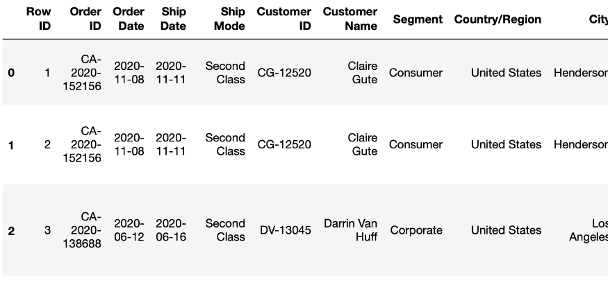
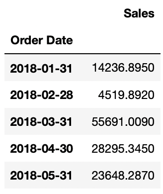
We only keep the date and sales columns to build time series objects. The following code sorts the sales figures in ascending order and summarizes the data by month.

#fetching required columns
data = superstore[['Order Date','Sales']] 
data = data.sort_values(by = 'Order Date')

#creating a ts object
data['Order Date'] = pd.to_datetime(data['Order Date'])
data.index = data['Order Date']
data = data.resample('M').sum()

We are going to visualize the time series:

import matplotlib.pyplot as plt
import seaborn as sns

plt.subplots(figsize = (17,7))
sns.lineplot(x = "Order Date", y = "Sales", data = data)
plt.show()

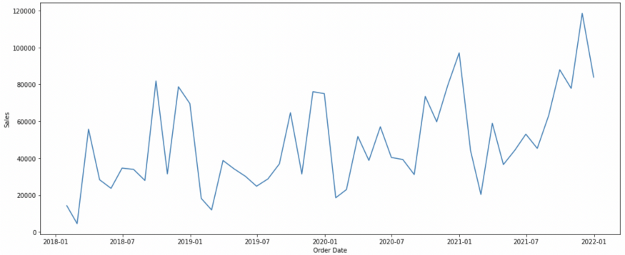
Above is our time series diagram. Time series has three important components: trend, seasonality and error. According to the properties of series and the assumptions we assume, we can regard series as an "addition model" or a "multiplication model".

Now, before switching to Tableau, I'll share the code I wrote to complete the model.

As mentioned at the beginning of this article, we will use three models. These are Holt linear model, Holt winter model and ARIMA. The first two methods are exponential smoothing method. Arima represents autoregressive comprehensive moving average, which is a regression method.

The following is the python code of Holt's Linear Method:

    import pandas as pd
    import numpy as np
    import statsmodels.api as sm
    from statsmodels.tsa.api import Holt
    import dateutil
    import datetime
    import warnings
    warnings.filterwarnings('ignore')
    
    superstore = pd.read_excel('/Users/jevpau1/Downloads/Python Notes-UT/Superstore.xls')
    
    #fetching required columns
    data = superstore[['Order Date','Sales']] 
    data = data.sort_values(by = 'Order Date')
    
    #creating a ts object
    data['Order Date'] = pd.to_datetime(data['Order Date'])
    data.index = data['Order Date']
    data = data.resample('M').sum()
    
    #use for training entire dataset
    data = data[:-(6)]
    
    #create future dataset
    step = dateutil.relativedelta.relativedelta(months=1)
    start = data.index[len(data)-1] + step
    index = pd.date_range(start, periods=6, freq='M')
    columns = ['Sales']
    df = pd.DataFrame(index=index, columns=columns)
    df = df.fillna(0)
   
    #Fit the model
    model = Holt(np.asarray(data['Sales'])).fit(smoothing_level = 0.3,smoothing_slope = 0.1)
    df['Sales']=model.forecast(6)
    df = df.fillna(0)
    x = pd.concat([data,df])
    x

The training time of the model is 42 months, and the last 6 months are used for prediction. Model parameters can be adjusted to accuracy. The model appends both and returns the entire series to us.

How do we relate it to Tableau?

Tableau has built-in analysis extensions that allow integration with other platforms.

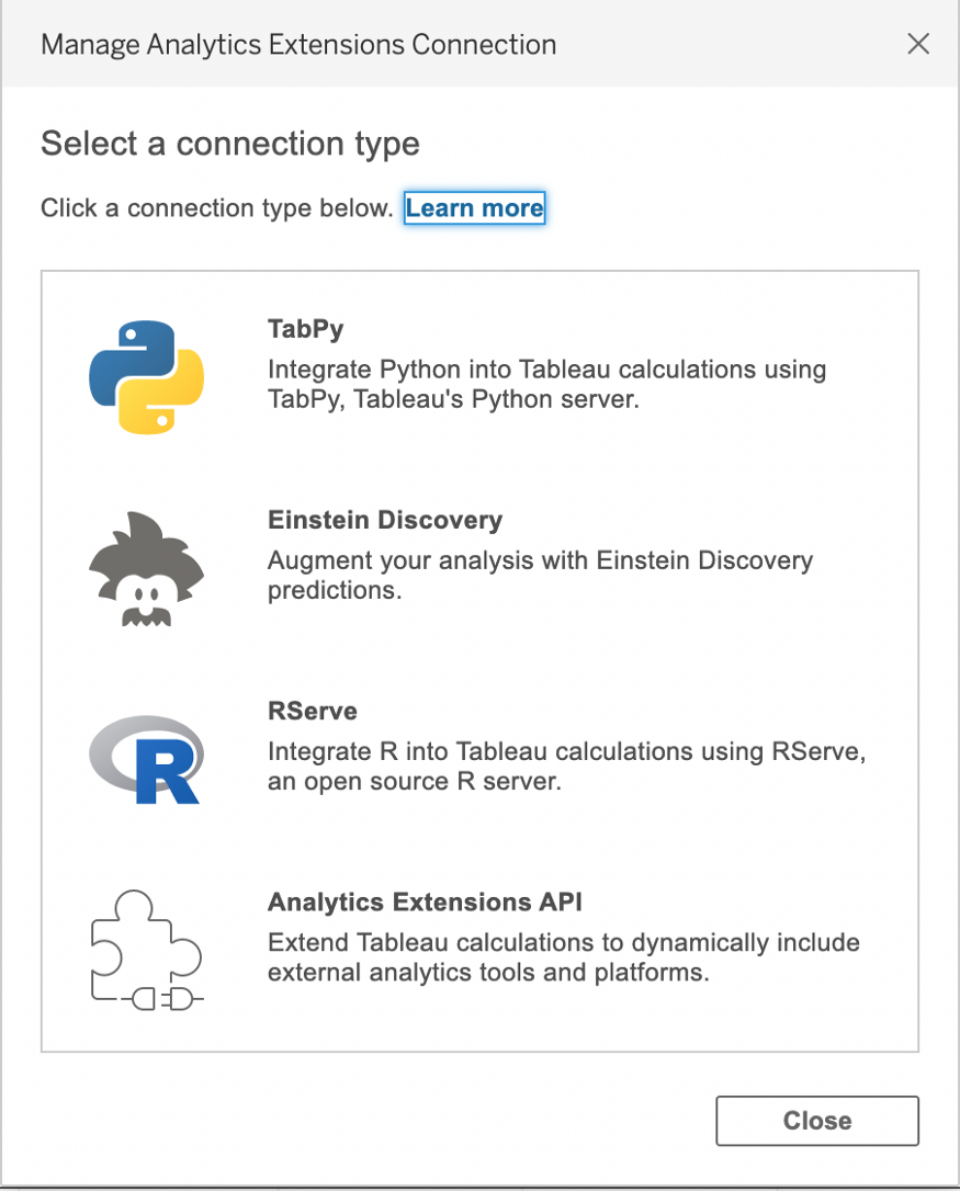
In this case, we select TabPy.

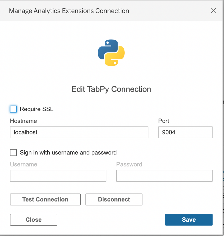
You can test the connection in Tableau in the pop-up window described above.

We also import TabPyClient in python environment to create connection objects.

import tabpy_client
connection = tabpy_client.Client('http://localhost:9004/')

Connect the model we just started with py to the tabserver.

Let's take a look at the modified code of Holt's Linear method, which can be deployed on TabPy.

Holt linear method

def holts_linear_method(_arg1,_arg2,_arg3):
    import pandas as pd
    from pandas import DataFrame
    import numpy as np
    import matplotlib.pyplot as plt
    import seaborn as sns
    from statsmodels.tsa.api import Holt
    import warnings
    import dateutil
    warnings.filterwarnings('ignore')
    
    data = DataFrame({'Period': _arg1,'Net Sales': _arg2})
    data = data.sort_values(by = 'Period')
    data['Period'] = pd.to_datetime(data['Period'])
    
    #use for training entire dataset
    data.index = pd.to_datetime(data['Period']) 
    data = data.resample('M').mean()
    data = data[:-(_arg3)]
    
    #create future dataset
    step = dateutil.relativedelta.relativedelta(months=1)
    start = data.index[len(data)-1] + step
    index = pd.date_range(start, periods=_arg3, freq='M')
    columns = ['Net Sales']
    df = pd.DataFrame(index=index, columns=columns)
    df = df.fillna(0)

    #Fit the model
    fit1 = Holt(np.asarray(data['Net Sales'])).fit(smoothing_level = 0.3,smoothing_slope = 0.1)
    df['Net Sales']=fit1.forecast(_arg3)
    df = df.fillna(0)
    x = pd.concat([data, df])
    return x['Net Sales'].tolist()

connection.deploy('Holt Linear Method',holts_linear_method,'Returns forecast of revenue', override=True)

We have created a function that returns the output of the model. Because we will read data from Tableau, we use the parameters that pass values from Tableau. You will notice that we use connection objects to deploy the model in TabPy. Similarly, you can create functions for other models.

Holt winter method

def holt_winters_method(_arg1,_arg2,_arg3):
    import pandas as pd
    from pandas import DataFrame
    import numpy as np
    import matplotlib.pyplot as plt
    import seaborn as sns
    from statsmodels.tsa.api import ExponentialSmoothing
    import warnings
    import dateutil
    warnings.filterwarnings('ignore')
   
    data = DataFrame({'Period': _arg1,'Net Sales': _arg2})
    data = data.sort_values(by = 'Period')
    data['Period'] = pd.to_datetime(data['Period'])
    
    #use for training entire dataset
    data.index = pd.to_datetime(data['Period']) 
    data = data.resample('M').mean()
    data = data[:-(_arg3)]
    
    #create future dataset
    step = dateutil.relativedelta.relativedelta(months=1)
    start = data.index[len(data)-1] + step
    index = pd.date_range(start, periods=_arg3, freq='M')
    columns = ['Net Sales']
    df = pd.DataFrame(index=index, columns=columns)
    df = df.fillna(0)
    
    #Fit Model
    fit1 = ExponentialSmoothing(np.asarray(data['Net Sales']) ,seasonal_periods=4 ,trend='add', seasonal='add',).fit()
    df['Net Sales']=fit1.forecast(_arg3)
    df = df.fillna(0)
    x = pd.concat([data, df])
    return x['Net Sales'].tolist()

connection.deploy('Holt Winters Method',holt_winters_method,'Returns forecast of revenue', override=True)

ARIMA

def sarima_method(_arg1,_arg2,_arg3):
    import pandas as pd
    from pandas import DataFrame
    import numpy as np
    import matplotlib.pyplot as plt
    import seaborn as sns
    import statsmodels.api as sm
    import dateutil
    import datetime
    import warnings
    warnings.filterwarnings('ignore')
    
    data = DataFrame({'Period': _arg1,'Net Sales': _arg2})
    data = data.sort_values(by = 'Period')
    data['Period'] = pd.to_datetime(data['Period'])
    
    #use for training entire dataset
    data.index = pd.to_datetime(data['Period']) 
    data = data.resample('M').mean()
    data = data[:-(_arg3)]
    
    #create future dataset
    step = dateutil.relativedelta.relativedelta(months=1)
    start = data.index[len(data)-1] + step
    index = pd.date_range(start, periods=_arg3, freq='M')
    columns = ['Net Sales']
    df = pd.DataFrame(index=index, columns=columns)
    df = df.fillna(0)
   
    #Fit the model
   
    fit1 = sm.tsa.statespace.SARIMAX(data['Net Sales'], order=(1, 1, 1),seasonal_order=(1,1,1,12)).fit()
    df['Net Sales']=fit1.forecast(_arg3)
    df = df.fillna(0)
    x = pd.concat([data, df])
    return x['Net Sales'].tolist()


connection.deploy('Seasonal ARIMA Method',sarima_method,'Returns forecast of revenue', override=True)

Now that we have deployed these models in TabPy, let's use it in Tableau. We will create a calculated field as follows:

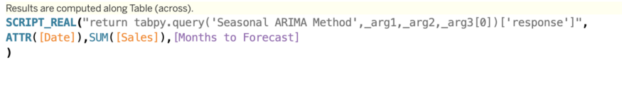
Tableau uses SCRIPT_REAL,SCRIPT_STR,SCRIPT_BOOL and SCRIPT_INT four functions return real, string, Boolean and integer types respectively. The above code tells tableau to run 'Seasonal ARIMA Method', which is deployed on TabPy, has three parameters (date, sales and month to forecast), and returns' response 'to the calculation field of tableau.

Similarly, we define calculation fields for the other two models. If we want to see it at a glance in Tableau, it will be like this:

Note that you can dynamically change the forecast period and view the forecast as needed. You want to choose the model that gives you the best accuracy. You can choose to create a parameter in Tableau to switch between models.

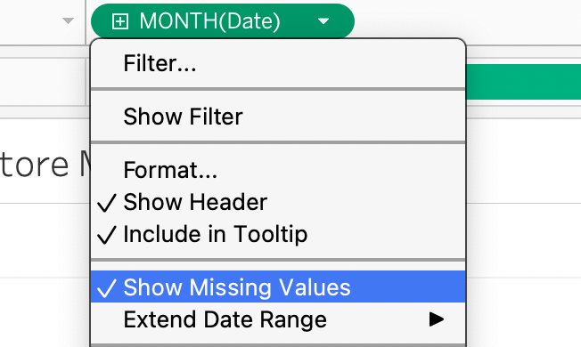
A key point to note is that we need to adapt to the prediction cycle in Tableau (in our example, in months) to make room for the value returned by TabPy. This is because when we pass the original dataset from Tableau, it does not have these empty records for future dates. The adjustment data I made are as follows:

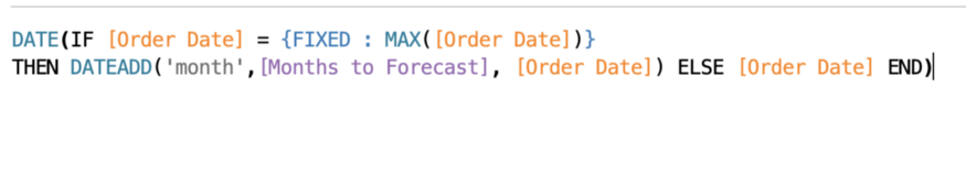
After adding the month to be predicted and passing it to TabPy, the above code actually extends the date range. In addition, we select "show missing values" as our date field.

As we extend the date range, the last date and sales figures will be pushed to the new forecast end date. However, we are only interested in forecasting; We can exclude this data point or use LAST()=FALSE in the filter box. You can come up with the same idea at will.

We have a good comprehensive prediction model in Tableau's visual discovery. You can definitely bring accuracy scores and model parameters to Tableau to make it cooler!

By Jerry Paul

Deep hub translation group