Paper core
target
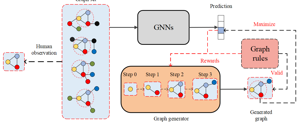
Here, the author aims at the graph classification problem of GNN. Study the model level interpretation method. The specific way is to train a graph generator
use f ( . ) f(.) f(.) Represents a trained GNN model. y ∈ c 1 , ⋅ ⋅ ⋅ , c ℓ y \in {c_1,···,c_ℓ} y ∈ c1, ⋅⋅⋅, c ℓ represents the label of the diagram. Given the trained GNN model f ( . ) f(.) f(.) And labels c i c_i ci . Graph generator generation can be predicted as c i c_i Graph of ci G ∗ G^* G∗. Defined as
G ∗ = a r g m a x G P ( f ( G ) = c i ) G^* = \mathop{argmax}\limits_{G}P(f(G) = c_i) G∗=GargmaxP(f(G)=ci)
That is, maximize G ∗ G^* G * is predicted to be c i c_i The probability of ci.
In the figure below, four graphs are predicted to be Category 3. Human beings have observed that a trigonometric graph is the common structure of the four graphs. The ultimate goal of graph generator is to generate similar graphs and introduce Graph rules (similar to manual verification) to enhance effectiveness.
Graph generator target
Represents the graph generator as g θ ( ⋅ ) g_\theta(·) g θ (⋅). Author passed T T T step s to generate G ∗ G^* G∗. t t The graph generated at time t is G t G_t Gt, including
- n t n_t nt # nodes
- Characteristic matrix X t ∈ R n t × d X_t \in R^{n_t \times d} Xt∈Rnt×d
- adjacency matrix A t ∈ { 0 , 1 } n t × n t A_t \in \{0,1\}^{n_t \times n_t} At∈{0,1}nt×nt
be
X
t
+
1
,
A
t
+
1
=
g
θ
(
X
t
,
A
t
)
X_{t+1},A_{t+1} = g_\theta(X_t,A_t)
Xt+1,At+1=gθ(Xt,At)
Generation task belongs to reinforcement learning task. Suppose the dataset exists k k k types of nodes, defining candidate set C = { s 1 , s 2 , ⋅ ⋅ ⋅ , s k } C = \{s_1,s_2,···,s_k\} C={s1,s2,⋅⋅⋅,sk}. For example, the node type in the chemical molecular graph is the atomic type, which has C = { carbon primary son , hydrogen primary son , ⋅ ⋅ ⋅ , oxygen primary son } C = \ {carbon atom, hydrogen atom, ···, oxygen atom \} C = {carbon atom, hydrogen atom, ⋅ ⋅, oxygen atom}. If the social network node has no classification, the candidate set has only one type.
g θ ( ⋅ ) g_\theta(·) g θ (⋅) by learning how to G t G_t Add edges to Gt G t + 1 G_{t+1} Gt+1. May be included in G t G_t Add an edge to the two nodes in Gt , or add a node from the candidate set.
Reinforcement learning tasks usually include four parts: state, action, policy and reward
-
state: t t The state at time t is the graph G t G_t Gt, the graph at the initial time can be composed of a node randomly selected from candidate set. It can also be selected manually. For example, carbon atoms are often selected as the initial time for the generation of organic structure diagram.
-
Action: t t The action at time t is recorded as a t a_t at. Graph based G t G_t Gt ^ generation G t + 1 G_{t + 1} The process of Gt+1. Specifically, it is to select an initial node and an end node and add an edge. Initial Node a t , s t a r t a_{t,start} at,start yes G t G_t The node in Gt , and the end node a t , e n d a_{t,end} at,end ; can be G t G_t Gt , or C C A node in C.
-
Policy: policy is the graph generator g θ ( ⋅ ) g_\theta(·) g θ (⋅) . It can be trained through reward mechanism and policy gradient.
-
reward: t t The reward at time t is expressed as R t R_t Rt. It includes 2 parts:
- From pre training GNN f ( . ) f(.) f(.) The guide will be increased g θ ( ⋅ ) g_\theta(·) g θ (⋅) the generated graph is classified as c i c_i The probability of ci. And use this probability as feedback update g θ ( ⋅ ) g_\theta(·) gθ(⋅).
- promote g θ ( ⋅ ) g_\theta(·) g θ (⋅) the generated graph is valid under graph rules. Graph rules include: two nodes in a social network cannot have multiple edges, and the degree of atoms in the molecular graph will not exceed its chemical valence.
Reward includes intermediate reward and global reward.
Graph generator
about t t t moment, action a t a_t at , recorded as ( a t , s t a r t , a t , e n d ) (a_{t,start}, a_{t,end}) (at,start,at,end). g θ ( ⋅ ) g_\theta(·) g θ (⋅) is based on G t G_t Gt , and C C C to predict the probability of different action s p t = ( p t , s t a r t , p t , e n d ) p_t=(p_{t,start} ,p_{t,end}) pt=(pt,start,pt,end). g θ ( ⋅ ) g_\theta(·) g θ (⋅) includes several GCN s.
The process can be described as
X
^
=
G
C
N
s
(
G
t
,
C
)
\widehat{X} = GCNs(G_t,C)
X
=GCNs(Gt,C)
p t , s t a r t = S o f t m a x ( M L P s ( X ^ ) ) p_{t,start} = Softmax(MLPs(\widehat{X})) pt,start=Softmax(MLPs(X ))
p t , e n d = S o f t m a x ( M L P s ( [ X ^ , x ^ s t a r t ) ) p_{t,end} = Softmax(MLPs([\widehat{X},\hat x_{start})) pt,end=Softmax(MLPs([X ,x^start))
among
- X ^ \widehat{X} X Node characteristics learned for GCNs
- a t , s t a r t ∼ p t , s t a r t ⊙ m t , s t a r t a_{t,start} ∼ p_{t,start} \odot m_{t,start} at,start∼pt,start⊙mt,start. m t , s t a r t m_{t,start} mt,start is a mask vector used to filter out the nodes in the candidate set, a t , s t a r t a_{t,start} at,start is used to select p t , s t a r t p_{t,start} Pt, the node with the highest probability in start
- x ^ s t a r t \hat x_{start} x^start is a t , s t a r t a_{t,start} Eigenvector of at,start +
- a t , e n d ∼ p t , e n d ⊙ m t , e n d a_{t,end} ∼ p_{t,end} \odot m_{t,end} at,end∼pt,end⊙mt,end. m t , e n d m_{t,end} mt,end , is a mask vector used to filter out nodes a t , s t a r t a_{t,start} at,start
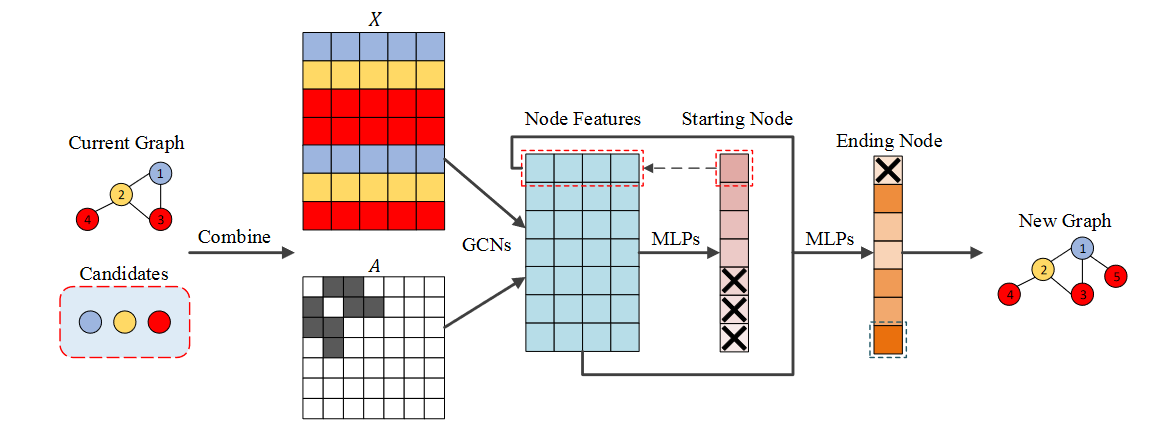
The example is shown in the figure below. Current Graph is G t G_t Gt. Can see G t G_t Gt # includes 4 nodes, and candidate set has 3 types of nodes. The generation process includes
- take G t G_t Characteristic matrix of Gt X t X_t Xt # and C C The feature vectors of nodes in C are concat enated to form the feature matrix X X X. And put G t G_t Adjacency matrix of Gt A t A_t At extended to A A A (from R 4 × 4 R^{4 \times 4} R4 × 4 expand into R 7 × 7 R^{7 \times 7} R7×7)
- The eigenvector of each node is formed through GCN X ^ \widehat{X} X (cyan matrix)
- X ^ \widehat{X} X Predict the start node of the newly added edge through the first MLPs a t , s t a r t a_{t,start} at,start × \times × The node of is the node mask ed. Can see C C All nodes in C are mask ed
- X ^ + x ^ s t a r t \widehat{X} + \hat x_{start} X +x^start predicts the end node of the new edge through the second MLPs a t , e n d a_{t,end} at,end. You can see that the starting node is mask ed.
- Formation diagram
G
t
+
1
G_{t + 1}
Gt+1. than
G
t
G_t
Gt # has one more node and one more edge.
Training chart generator
train
g
θ
(
⋅
)
g_\theta(·)
g θ (⋅) policy gradient is used. The formula is
L
g
=
−
R
t
(
L
C
E
(
p
t
,
s
t
a
r
t
,
a
t
,
s
t
a
r
t
)
+
L
C
E
(
p
t
,
e
n
d
,
a
t
,
e
n
d
)
)
\mathcal{L}_g = -R_t(\mathcal{L}_{CE}(p_{t,start}, a_{t,start}) + \mathcal{L}_{CE}(p_{t,end}, a_{t,end}))
Lg=−Rt(LCE(pt,start,at,start)+LCE(pt,end,at,end))
among
- L C E \mathcal{L}_{CE} LCE = cross entropy loss
- R t R_t Rt ^ is t t t time reward function
R t R_t Rt includes R t , f R_{t,f} Rt,f , and R t , r R_{t,r} Rt,r # 2 parts.
R t , f ( G t + 1 ) = p ( f ( G t + 1 ) = c i ) − 1 / ℓ R_{t,f}(G_{t+1}) = p(f(G_{t+1})=ci) − 1 / ℓ Rt,f(Gt+1)=p(f(Gt+1)=ci)−1/ℓ
R t , f = R t , f ( G t + 1 ) + λ 1 . ∑ i = 0 m R t , f ( R o l l o u t ( G t + 1 ) ) m R_{t,f} = R_{t,f}(G_{t+1}) + \lambda_1 . \frac{\sum_{i = 0}^m R_{t,f}(Rollout(G_{t+1}))}{m} Rt,f=Rt,f(Gt+1)+λ1.m∑i=0mRt,f(Rollout(Gt+1))
R t = R t , f ( G t + 1 ) + λ 1 . ∑ i = 0 m R t , f ( R o l l o u t ( G t + 1 ) ) m + λ 2 . R t , r R_t = R_{t,f}(G_{t+1}) + \lambda_1 . \frac{\sum_{i = 0}^m R_{t,f}(Rollout(G_{t+1}))}{m} + \lambda_2.R_{t,r} Rt=Rt,f(Gt+1)+λ1.m∑i=0mRt,f(Rollout(Gt+1))+λ2.Rt,r
among
- ℓ ℓ ℓ is the number of labels in the figure
- λ 1 \lambda_1 λ 1. And λ 2 \lambda_2 λ 2 ¢ is a super parameter
- R t , r R_{t,r} Rt,r , stands for manually formulated graph rules. For example, each node of the molecular graph must meet the rules of chemical bond (it must be legal organic matter), otherwise R t , r R_{t,r} Rt,r , will be negative
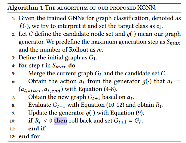 The most important ones in this algorithm are 8, 9 and 10 lines.
experiment
data set
The author uses the synthetic data set Is_Acyclic and real data set MUTAG. Here I use MUTAG to reproduce.
The MUTAG dataset is divided into two categories according to their mutagenic effects on bacteria. Node types include Carbon, Nitrogen, Oxygen, Fluorine, Iodine, Chlorine, and Bromine. The type of edge is not used here.
MUTAG includes 188 molecular diagrams, a total of 3371 nodes (atoms) and 7442 edges (chemical bonds). The data set directory is as follows
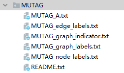
- node_labels.txt records the type of each node in 3371 nodes (numbered from 0 to 6)
- graph_indicator.txt record the corresponding index number of each node (the index number is numbered from 1-188)
- graph_labels.txt records the corresponding type of 188 graphs (label is 1 or - 1)
- A.txt records 7442 edges with (start_node_idx,end_node_idx), start_ node_ IDX and end_ node_ IDX is in the range of 3371
- edge_labels.txt records 7442 edges and the type of each edge, which is not used here.
The code for loading the dataset is as follows:
import numpy as np
import scipy.sparse as sp
import torch

def encode_onehot(labels):
    classes = set(labels)
    classes_dict = {c: np.identity(len(classes))[i, :] for i, c in
                    enumerate(classes)}
    labels_onehot = np.array(list(map(classes_dict.get, labels)),
                             dtype=np.int32)
    return labels_onehot


def normalize(mx):
    """Row-normalize sparse matrix"""
    rowsum = np.array(mx.sum(1))
    r_inv = np.power(rowsum, -1).flatten()
    r_inv[np.isinf(r_inv)] = 0.
    r_mat_inv = sp.diags(r_inv)
    mx = r_mat_inv.dot(mx)
    return mx

def load_split_MUTAG_data(path="datas/MUTAG/", dataset="MUTAG_", split_train=0.7, split_val=0.15):
    """Load MUTAG data """
    print('Loading {} dataset...'.format(dataset))

    # Load the label of the graph
    graph_labels = np.genfromtxt("{}{}graph_labels.txt".format(path, dataset),
                           dtype=np.dtype(int))
    graph_labels = encode_onehot(graph_labels)  # (188, 2)
    graph_labels = torch.LongTensor(np.where(graph_labels)[1]) # (188, 1)


    # Index number of graph node
    graph_idx = np.genfromtxt("{}{}graph_indicator.txt".format(path, dataset),
                              dtype=np.dtype(int))

    graph_idx = np.array(graph_idx, dtype=np.int32)
    idx_map = {j: i for i, j in enumerate(graph_idx)} # key, value indicates the starting node of the key graph, and the index number is value
    length = len(idx_map.keys()) # How many pictures are there altogether
    num_nodes = [idx_map[n] - idx_map[n - 1] if n - 1 > 1 else idx_map[n] for n in range(1, length + 1)] # A list with a length of 188 indicates how many nodes there are in each graph
    max_num_nodes = max(num_nodes) # How many nodes does the largest graph have
    features_list = []
    adj_list = []
    prev = 0

    # Label of node
    nodeidx_features = np.genfromtxt("{}{}node_labels.txt".format(path, dataset), delimiter=",",
                                     dtype=np.dtype(int))
    node_features = np.zeros((nodeidx_features.shape[0], max(nodeidx_features) + 1))
    node_features[np.arange(nodeidx_features.shape[0]), nodeidx_features] = 1

    # Edge information
    edges_unordered = np.genfromtxt("{}{}A.txt".format(path, dataset), delimiter=",",
                                    dtype=np.int32)

    # Label of edge
    edges_label = np.genfromtxt("{}{}edge_labels.txt".format(path, dataset), delimiter=",",
                                dtype=np.int32)  # shape = (7442,)

    # Generate adjacency matrix A, which includes all edges in the dataset
    adj = sp.coo_matrix((edges_label, (edges_unordered[:, 0] - 1, edges_unordered[:, 1] - 1)))

    # In the paper, a ^ = (d ~) ^ 0.5 is the formula of a ~ (d ~) ^ 0.5
    adj = adj + adj.T.multiply(adj.T > adj) - adj.multiply(adj.T > adj)

    node_features = normalize(node_features)
    adj = normalize(adj + sp.eye(adj.shape[0])) # Corresponding formula A~=A+IN
    adj = adj.todense()

    for n in range(1, length + 1):
        # entry is the characteristic matrix X of the nth graph
        entry = np.zeros((max_num_nodes, max(nodeidx_features) + 1))
        entry[:idx_map[n] - prev] = node_features[prev:idx_map[n]]
        entry = torch.FloatTensor(entry)
        features_list.append(entry.tolist())

        # entry is the adjacency matrix A of the nth graph
        entry = np.zeros((max_num_nodes, max_num_nodes))
        entry[:idx_map[n] - prev, :idx_map[n] - prev] = adj[prev:idx_map[n], prev:idx_map[n]]
        entry = torch.FloatTensor(entry)
        adj_list.append(entry.tolist())

        prev = idx_map[n] # prev is the index number of the starting node of the next graph

    num_total = max(graph_idx)
    num_train = int(split_train * num_total)
    num_val = int((split_train + split_val) * num_total)

    if (num_train == num_val or num_val == num_total):
        return

    features_list = torch.FloatTensor(features_list)
    adj_list = torch.FloatTensor(adj_list)

    idx_train = range(num_train)
    idx_val = range(num_train, num_val)
    idx_test = range(num_val, num_total)

    idx_train = torch.LongTensor(idx_train)
    idx_val = torch.LongTensor(idx_val)
    idx_test = torch.LongTensor(idx_test)

    # The return value is the adjacency matrix list of 188 graphs, the characteristic matrix list of 188 graphs, the label of 188 graphs, the index number of the starting node of each graph, the index number of the training set,
    # Validate set index number, test set index number
    return adj_list, features_list, graph_labels, idx_map, idx_train, idx_val, idx_test
Here are 188 graphs, and the adjacency matrix dimension of each graph is m a x _ n o d e _ n u m × m a x _ n o d e _ n u m max\_node\_num \times max\_node\_num max_node_num × max_node_num. The dimension of characteristic matrix is m a x _ n o d e _ n u m × f e a t u r e _ d i m max\_node\_num \times feature\_dim max_node_num×feature_dim
Training GCN classifier
here f ( . ) f(.) f(.) Represented by GCN, the code of the model is as follows
import math

import torch
import torch.nn as nn
import torch.nn.functional as F
from torch.nn.parameter import Parameter


class GraphConvolution(nn.Module):
    """
    Simple GCN layer, similar to https://arxiv.org/abs/1609.02907
    paper: Semi-Supervised Classification with Graph Convolutional Networks
    """
    # The parameters of the model include weight and bias
    def __init__(self, in_features, out_features):
        super(GraphConvolution, self).__init__()
        self.in_features = in_features
        self.out_features = out_features
        self.weight = Parameter(torch.FloatTensor(in_features, out_features))
        self.bias = Parameter(torch.FloatTensor(out_features))
        self.reset_parameters()

    # Weight initialization
    def reset_parameters(self):
        stdv = 1. / math.sqrt(self.weight.size(1))
        self.weight.data.uniform_(-stdv, stdv)
        self.bias.data.uniform_(-stdv, stdv)

    # Similar to tostring
    def __repr__(self):
        return self.__class__.__name__ + ' (' \
               + str(self.in_features) + ' -> ' \
               + str(self.out_features) + ')'

    # Calculate A~ X W(0)
    def forward(self, input, adj):
        # input.shape = [max_node, features] = X
        # adj.shape = [max_node, max_node] = A~
        # torch.mm(a, b) is the multiplication of matrix A and matrix B, torch Mul (a, b) is the multiplication of the corresponding bits of matrices A and B, and the dimensions of a and B must be equal
        support = torch.mm(input, self.weight)
        output = torch.spmm(adj, support)
        return output + self.bias


class GCN(nn.Module):
    # Number of feature s; Final classification number

    def __init__(self, nfeat, nclass, dropout):
        """ As per paper """
        """ 3 layers of GCNs with output dimensions equal to 32, 48, 64 respectively and average all node features """
        """ Final classifier with 2 fully connected layers and hidden dimension set to 32 """
        """ Activation function - ReLu (Mutag) """
        super(GCN, self).__init__()

        self.dropout = dropout

        self.gc1 = GraphConvolution(nfeat, 32)
        self.gc2 = GraphConvolution(32, 48)
        self.gc3 = GraphConvolution(48, 64)
        self.fc1 = nn.Linear(64, 32)
        self.fc2 = nn.Linear(32, nclass)

    def forward(self, x, adj):
        # x.shape = [max_node, features]
        # adj.shape = [max_node, max_node]
        x = F.relu(self.gc1(x, adj))
        x = F.dropout(x, self.dropout, training=self.training)
        x = F.relu(self.gc2(x, adj))
        x = F.dropout(x, self.dropout, training=self.training)
        x = F.relu(self.gc3(x, adj))


        y = torch.mean(x, 0)  # mean is used as the aggregation function to aggregate the characteristics of all nodes
        y = F.relu(self.fc1(y))
        y = F.dropout(y, self.dropout, training=self.training)
        y = F.softmax(self.fc2(y), dim=0)

        return y
Training GCN classifier
from Load_dataset import load_split_MUTAG_data, accuracy
from Model import GCN
import time

import numpy as np
import torch
import torch.optim as optim
import torch.nn.functional as F

model_path = 'model/gcn_first.pth'

epochs = 1000
seed = 200
lr = 0.001
dropout = 0.1
weight_decay = 5e-4

np.random.seed(seed)
torch.manual_seed(seed)
torch.cuda.manual_seed(seed)


class EarlyStopping():
    def __init__(self, patience=10, min_loss=0.5, hit_min_before_stopping=False):
        self.patience = patience
        self.counter = 0
        self.hit_min_before_stopping = hit_min_before_stopping
        if hit_min_before_stopping:
            self.min_loss = min_loss
        self.best_loss = None
        self.early_stop = False

    def __call__(self, loss):
        if self.best_loss is None:
            self.best_loss = loss
        elif loss > self.best_loss:
            self.counter += 1
            if self.counter > self.patience:
                if self.hit_min_before_stopping == True and loss > self.min_loss:
                    print("Cannot hit mean loss, will continue")
                    self.counter -= self.patience
                else:
                    self.early_stop = True
        else:
            self.best_loss = loss
            counter = 0


if __name__ == '__main__':
    # adj_list: [188, 29, 29]
    # features_list: [188, 29, 7]
    # graph_labels: [188]
    adj_list, features_list, graph_labels, idx_map, idx_train, idx_val, idx_test = load_split_MUTAG_data()
    idx_train = torch.cat([idx_train, idx_val, idx_test])

    model = GCN(nfeat=features_list[0].shape[1], # nfeat = 7
                nclass=graph_labels.max().item() + 1, # nclass = 2
                dropout=dropout)
    optimizer = optim.Adam(model.parameters(),
                           lr=lr, weight_decay=weight_decay)

    model.cuda()
    features_list = features_list.cuda()
    adj_list = adj_list.cuda()
    graph_labels = graph_labels.cuda()
    idx_train = idx_train.cuda()
    idx_val = idx_val.cuda()
    idx_test = idx_test.cuda()

    # Training model
    early_stopping = EarlyStopping(10, hit_min_before_stopping=True)
    t_total = time.time()

    for epoch in range(epochs):
        t = time.time()
        model.train()
        optimizer.zero_grad()

        # # Split
        outputs = []
        for i in idx_train:
            output = model(features_list[i], adj_list[i])
            output = output.unsqueeze(0)
            outputs.append(output)
        output = torch.cat(outputs, dim=0)


        loss_train = F.cross_entropy(output, graph_labels[idx_train])
        acc_train = accuracy(output, graph_labels[idx_train])
        loss_train.backward()
        optimizer.step()

        model.eval()
        outputs = []
        for i in idx_val:
            output = model(features_list[i], adj_list[i])
            output = output.unsqueeze(0)
            outputs.append(output)
        output = torch.cat(outputs, dim=0)
        loss_val = F.cross_entropy(output, graph_labels[idx_val])
        acc_val = accuracy(output, graph_labels[idx_val])

        print('Epoch: {:04d}'.format(epoch + 1),
              'loss_train: {:.4f}'.format(loss_train.item()),
              'acc_train: {:.4f}'.format(acc_train.item()),
              'loss_val: {:.4f}'.format(loss_val.item()),
              'acc_val: {:.4f}'.format(acc_val.item()),
              'time: {:.4f}s'.format(time.time() - t))

        print(loss_val)
        early_stopping(loss_val)
        if early_stopping.early_stop == True:
            break

    print("Optimization Finished!")
    print("Total time elapsed: {:.4f}s".format(time.time() - t_total))

    torch.save(model.state_dict(), model_path)
Training chart generator
Class definition of generator
import random
import copy
import numpy as np
import torch
import torch.nn as nn
import torch.nn.functional as F
from Model import GraphConvolution, GCN
rollout = 10
max_gen_step = 10
MAX_NUM_NODES = 28 # for mutag
random.seed(200)
class Generator(nn.Module):
def __init__(self, model_path: str, C: list, node_feature_dim: int ,num_class = 2, c=0, hyp1=1, hyp2=2, start=None, nfeat=7, dropout=0.1):
"""
:param C: Candidate set of nodes (list)
:param start: Starting node (defaults to randomised node)
"""
super(Generator, self).__init__()
self.nfeat = nfeat
self.dropout = dropout
self.c = c
self.fc = nn.Linear(nfeat, 8)
self.gc1 = GraphConvolution(8, 16)
self.gc2 = GraphConvolution(16, 24)
self.gc3 = GraphConvolution(24, 32)
# MLP1
# 2 FC layers with hidden dimension 16
self.mlp1 = nn.Sequential(nn.Linear(32, 16), nn.Linear(16, 1))
# MLP2
# 2 FC layers with hidden dimension 24
self.mlp2 = nn.Sequential(nn.Linear(64, 24), nn.Linear(24, 1))
# Hyperparameters
self.hyp1 = hyp1
self.hyp2 = hyp2
self.candidate_set = C
# Default starting node (if any)
if start is not None:
self.start = start
self.random_start = False
else:
self.start = random.choice(np.arange(0, len(self.candidate_set)))
self.random_start = True
# Load GCN for calculating reward
self.model = GCN(nfeat=node_feature_dim,
nclass=num_class,
dropout=dropout)
self.model.load_state_dict(torch.load(model_path))
for param in self.model.parameters():
param.requires_grad = False
self.reset_graph()
def reset_graph(self):
"""
Reset g.G to default graph with only start node, Generate a graph with only one node
"""
if self.random_start == True:
self.start = random.choice(np.arange(0, len(self.candidate_set)))
# The initial graph is masked except for the first node, where the side length of the adjacency matrix is MAX_NUM_NODES + len(self.candidate_set), so the mask is not only the candidate assembly point, but also all virtual nodes in the figure
mask_start = torch.BoolTensor(
[False if i == 0 else True for i in range(MAX_NUM_NODES + len(self.candidate_set))])
adj = torch.zeros((MAX_NUM_NODES + len(self.candidate_set), MAX_NUM_NODES + len(self.candidate_set)),
dtype=torch.float32) # Here, the adj shape is [max_num_nodes + len (self. Candidate_set), and there may be empty nodes in the middle of max_num_nodes + len (self. Candidate_set)]
feat = torch.zeros((MAX_NUM_NODES + len(self.candidate_set), len(self.candidate_set)), dtype=torch.float32)
feat[0, self.start] = 1
feat[np.arange(-len(self.candidate_set), 0), np.arange(0, len(self.candidate_set))] = 1
degrees = torch.zeros(MAX_NUM_NODES)
self.G = {'adj': adj, 'feat': feat, 'degrees': degrees, 'num_nodes': 1, 'mask_start': mask_start}
## Calculate GT - > GT + 1
def forward(self, G_in):
## G_in is Gt
G = copy.deepcopy(G_in)
x = G['feat'].detach().clone() # Characteristic matrix of Gt
adj = G['adj'].detach().clone() # Adjacency matrix of Gt
## Corresponding X = GCNs(Gt, C)
x = F.relu6(self.fc(x))
x = F.dropout(x, self.dropout, training=self.training)
x = F.relu6(self.gc1(x, adj))
x = F.dropout(x, self.dropout, training=self.training)
x = F.relu6(self.gc2(x, adj))
x = F.dropout(x, self.dropout, training=self.training)
x = F.relu6(self.gc3(x, adj))
x = F.dropout(x, self.dropout, training=self.training)
## pt,start=Softmax(MLPs(X))
p_start = self.mlp1(x)
p_start = p_start.masked_fill(G['mask_start'].unsqueeze(1), 0)
p_start = F.softmax(p_start, dim=0)
a_start_idx = torch.argmax(p_start.masked_fill(G['mask_start'].unsqueeze(1), -1))
## pt,end=Softmax(MLPs([X,x^start))
# broadcast
x1, x2 = torch.broadcast_tensors(x, x[a_start_idx])
x = torch.cat((x1, x2), 1) # cat increases dim from 32 to 64
# Calculate maskt and end. Except for the nodes in the candidate set and Gt nodes that are not selected as the initial nodes, others are masked
mask_end = torch.BoolTensor([True for i in range(MAX_NUM_NODES + len(self.candidate_set))])
mask_end[MAX_NUM_NODES:] = False
mask_end[:G['num_nodes']] = False
mask_end[a_start_idx] = True
p_end = self.mlp2(x)
p_end = p_end.masked_fill(mask_end.unsqueeze(1), 0)
p_end = F.softmax(p_end, dim=0)
a_end_idx = torch.argmax(p_end.masked_fill(mask_end.unsqueeze(1), -1))
# Return new G
# If a_end_idx is not masked, node exists in graph, no new node added
if G['mask_start'][a_end_idx] == False:
G['adj'][a_end_idx][a_start_idx] += 1
G['adj'][a_start_idx][a_end_idx] += 1
# Update degrees
G['degrees'][a_start_idx] += 1
G['degrees'][G['num_nodes']] += 1
else:
# Add node
G['feat'][G['num_nodes']] = G['feat'][a_end_idx]
# Add edge
G['adj'][G['num_nodes']][a_start_idx] += 1
G['adj'][a_start_idx][G['num_nodes']] += 1
# Update degrees
G['degrees'][a_start_idx] += 1
G['degrees'][G['num_nodes']] += 1
# Update start mask
G_mask_start_copy = G['mask_start'].detach().clone()
G_mask_start_copy[G['num_nodes']] = False
G['mask_start'] = G_mask_start_copy
G['num_nodes'] += 1
return p_start, a_start_idx, p_end, a_end_idx, G
Based on the forward function G t G_t Gt calculation G t + 1 G_{t+1} The process of Gt+1. Here, the maximum number of nodes in a graph in the classification task is defined_ NUM_ NODES = 28. And candidate set C C C has 7 nodes. from G t G_t Gt # to G t + 1 G_{t+1} The side lengths of Gt+1 ﹐ adjacency matrix are MAX_NUM_NODES + len(candidate set) = 35. That is, there are many virtual nodes in the middle (similar to padding). So you have to consider this when you mask.
The reward function is defined as follows:
### reward function
    def calculate_reward(self, G_t_1):
        """
        Rtr     Calculated from graph rules to encourage generated graphs to be valid
                1. Only one edge to be added between any two nodes
                2. Generated graph cannot contain more nodes than predefined maximum node number
                3. (For chemical) Degree cannot exceed valency
                If generated graph violates graph rule, Rtr = -1

        Rtf     Feedback from trained model
        """

        rtr = self.check_graph_rules(G_t_1)

        rtf = self.calculate_reward_feedback(G_t_1)
        rtf_sum = 0
        for m in range(rollout):
            p_start, a_start, p_end, a_end, G_t_1 = self.forward(G_t_1)
            rtf_sum += self.calculate_reward_feedback(G_t_1)
        rtf = rtf + rtf_sum * self.hyp1 / rollout

        return rtf + self.hyp2 * rtr

    def calculate_reward_feedback(self, G_t_1):
        """
        p(f(G_t_1) = c) - 1/l
        where l denotes number of possible classes for f
        """
        f = self.model(G_t_1['feat'], G_t_1['adj'], None)
        return f[self.c] - 1 / len(f)


    ## graph rules
    def check_graph_rules(self, G_t_1):
        """
        For mutag, node degrees cannot exceed valency
        """
        idx = 0

        for d in G_t_1['degrees']:
            if d is not 0:
                node_id = torch.argmax(G_t_1['feat'][idx])  # Eg. [0, 1, 0, 0] -> 1
                node = self.candidate_set[node_id]  # Eg ['C.4', 'F.2', 'Br.7'][1] = 'F.2'
                max_valency = int(node.split('.')[1])  # Eg. C.4 -> ['C', '4'] -> 4

                # If any node degree exceeds its valency, return -1
                if max_valency < d:
                    return -1

        return 0
Can see
- graph rules only detects whether the degree of a node exceeds its atomic chemical valence. If it is illegal, it returns - 1 and if it is legal, it returns 0
loss is
## Calculate loss
    def calculate_loss(self, Rt, p_start, a_start, p_end, a_end, G_t_1):
        """
        Calculated from cross entropy loss (Lce) and reward function (Rt)
        where loss = -Rt*(Lce_start + Lce_end)
        """

        Lce_start = F.cross_entropy(torch.reshape(p_start, (1, 35)), a_start.unsqueeze(0))
        Lce_end = F.cross_entropy(torch.reshape(p_end, (1, 35)), a_end.unsqueeze(0))

        return -Rt * (Lce_start + Lce_end)
- 35 is MAX_NUM_NODES + len(candidate set) = 35.
Here, reward and loss are both member functions of the Generator class.
Training code
from GraphGenerator import Generator
import copy

import numpy as np
import networkx as nx
import matplotlib.pyplot as plt

import torch
import torch.optim as optim

lr = 0.01
b1 = 0.9
b2 = 0.99
hyp1 = 1
hyp2 = 2
max_gen_step = 10  # T = 10

candidate_set = ['C.4', 'N.5', 'O.2', 'F.1', 'I.7', 'Cl.7', 'Br.5']  # C.4 indicates that the degree of carbon atom does not exceed 4
model_path = 'model/gcn_first.pth'

## Training generator
def train_generator(c=0, max_nodes=5):
    g.c = c
    for i in range(max_gen_step):
        optimizer.zero_grad()
        G = copy.deepcopy(g.G)
        p_start, a_start, p_end, a_end, G = g.forward(G)

        Rt = g.calculate_reward(G)
        loss = g.calculate_loss(Rt, p_start, a_start, p_end, a_end, G)
        loss.backward()
        optimizer.step()

        if G['num_nodes'] > max_nodes:
            g.reset_graph()
        elif Rt > 0:
            g.G = G


## Generate graph
def generate_graph(c=0, max_nodes=5):
    g.c = c
    g.reset_graph()

    for i in range(max_gen_step):
        G = copy.deepcopy(g.G)
        p_start, a_start, p_end, a_end, G = g.forward(G)
        Rt = g.calculate_reward(G)

        if G['num_nodes'] > max_nodes:
            return g.G
        elif Rt > 0:
            g.G = G

    return g.G

## Draw a picture
def display_graph(G):
    G_nx = nx.from_numpy_matrix(np.asmatrix(G['adj'][:G['num_nodes'], :G['num_nodes']].numpy()))
    # nx.draw_networkx(G_nx)

    layout=nx.spring_layout(G_nx)
    nx.draw(G_nx, layout)

    coloring=torch.argmax(G['feat'],1)
    colors=['b','g','r','c','m','y','k']

    for i in range(7):
        nx.draw_networkx_nodes(G_nx,pos=layout,nodelist=[x for x in G_nx.nodes() if coloring[x]==i],node_color=colors[i])
        nx.draw_networkx_labels(G_nx,pos=layout,labels={x:candidate_set[i].split('.')[0] for x in G_nx.nodes() if coloring[x]==i})
    nx.draw_networkx_edges(G_nx,pos=layout,width=list(nx.get_edge_attributes(G_nx,'weight').values()))
    nx.draw_networkx_edge_labels(G_nx,pos=layout,edge_labels=nx.get_edge_attributes(G_nx, "weight"))

    plt.show()

if __name__ == '__main__':
    g = Generator(model_path = model_path, C = candidate_set, node_feature_dim=7 ,c=0, start=0)
    optimizer = optim.Adam(g.parameters(), lr=lr, betas=(b1, b2))

    for i in range(1, 10):
        ## Generate a graph structure with up to i nodes respectively
        g.reset_graph()
        train_generator(c=1, max_nodes=i)
        to_display = generate_graph(c=1, max_nodes=i)
        display_graph(to_display)
        print(g.model(to_display['feat'], to_display['adj']))
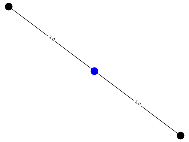
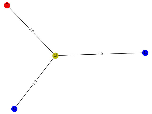
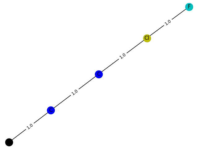
The training process here cannot be evaluated with data, but can only be drawn. Here, GCN classification models containing 1-9 nodes are generated respectively f ( . ) f(.) f(.) The subgraph structure with 1 is predicted and the probability of 1 is given. give the result as follows
1 probability: 0.7715
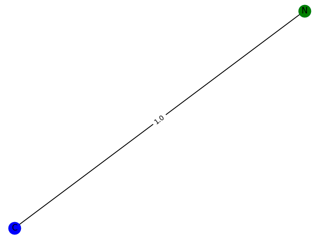
2. Probability: 0.7935

3. Probability: 0.8358
4 probability: 0.8556
5 probability: 0.8778
6 probability: 0.8533
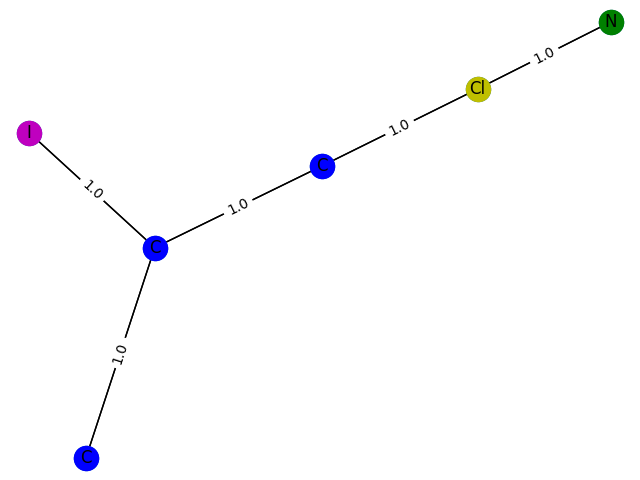
7 probability: 0.9010
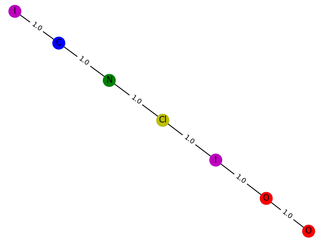
8 probability: 0.9005
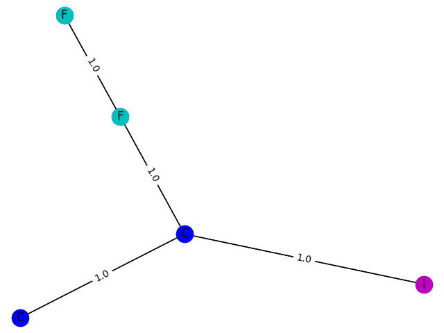
9 probability: 0.8510
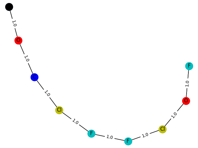
The gap with the paper is still quite obvious. The adjustment of parameters is still very learned. Maybe I'm too good to master.