reference resources:
Finally write the summary of XGBoost!
XGBoost of machine learning algorithm and its automatic parameter adjustment
reference resources: How does xgboost handle missing values
introduce
In 2016, an extensible machine learning system was developed under the leadership of Chen Tianqi of the University of Washington. Strictly speaking, XGBoost is not a model, but a software package for users to easily solve classification, regression or sorting problems. The gradient lifting tree (GBDT) model is implemented internally, and many algorithms in the model are optimized, which not only achieves high precision, but also maintains a very fast speed.
principle
First, let's talk about GBDT, which is an addition model based on boosting enhancement strategy. During training, the forward greedy algorithm is used for learning. Each iteration learns a CART tree to fit the residual between the prediction result of the previous t-1 tree and the real value of the training sample. XGBoost is a series of optimizations based on GBDT, such as second-order Taylor expansion of loss function, addition of regular term to objective function, support for parallel and automatic processing of missing values, etc., but there is no significant change in their core ideas.
XGBOOST is famous for its Regularized Boosting technology. It controls the complexity of the model and prevents over fitting by adding regularization terms to the cost function. Parallel processing can be realized, which has a great speed improvement compared with GBM.
XGBOOST objective function:
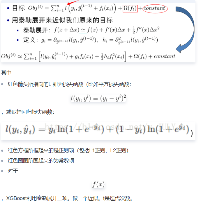
It can be clearly seen that the final objective function only depends on the first and second derivatives of each data point on the error function
advantage
Advantages of XGBoost:
-
Regularization: it can effectively prevent over fitting of the model
-
Parallel processing: XGBoost processes data in parallel faster than ordinary lifting trees
Faster algorithm -
Automatic processing of missing data: do not make segmentation points, but put the missing values into the left and right subtrees to see the effect
-
Pruning strategy: ordinary promotion adopts greedy algorithm, only when there is no more
The splitting will stop when the gain is -
You can continue to iterate on the current tree model: xGBoost can use different iteration strategies in training
Compared with GBDT model, XGBoost adopts the following optimization:
- Taylor's second-order expansion of the objective function can more efficiently fit the error.
- An algorithm for estimating split points is proposed to speed up the construction of CART tree and deal with sparse data at the same time.
- A tree parallel strategy is proposed to speed up the iteration.
- The distributed algorithm of the model is optimized.
Comparison with other algorithms
GBDT

Random forest
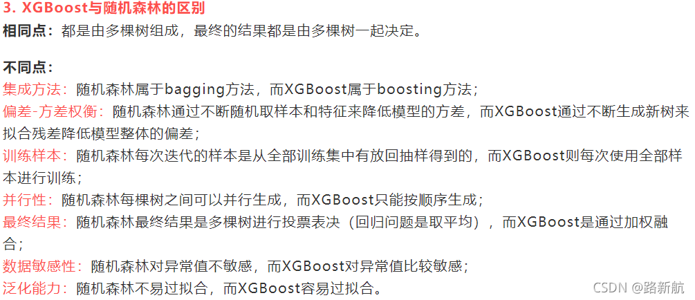
Other integrated learning algorithms
On the one hand, XGBoost improves the robustness of the model by introducing regular terms and column sampling. On the other hand, XGBoost adopts the parallelization strategy when selecting the splitting point of each tree, which greatly improves the running speed of the model.
Parameters and tuning parameters
Important parameters
params = {
    'booster':'gbtree', # gblinear
    'objective':'multi:softmax',   # Multi classification problem
    'num_class':10,  # Number of categories, used with multi softmax
    'gamma':0.1,    # The larger the parameter used to control whether to post prune, the more conservative it is. It is generally 0.1 0.2
    'max_depth':12,  # The greater the depth of the construction tree, the easier it is to over fit
    'lambda':2,  # The L2 regularization term parameter of the weight value controlling the complexity of the model. The larger the parameter, the less easy it is to over fit the model
    'subsample':0.7, # Random sampling training samples
    'colsample_bytree':3,# This parameter defaults to 1, which is the sum of h in each leaf
    # For the 0-1 classification when the positive and negative samples are unbalanced, it is assumed that h is near 0.01, min_child_weight is 1
    #This means that the leaf node needs to contain at least 100 samples. This parameter greatly affects the results,
    # Controls the minimum value of the sum of the second derivative in the leaf node. The smaller the parameter value, the easier it is to over fit
    'silent':0,  # If it is set to 1, there is no operation information input, preferably set to 0
    'eta':0.007,  # Like learning rate
    'seed':1000,
    'nthread':7,  #Number of CPU threads
    #'eval_metric':'auc'
}
Parameter classification
The model parameters are divided into three categories: general parameters, Booster parameters and objective function parameters.
General parameters
General parameters are the macro parameters of the model, which usually do not need to be set deliberately.
1. The booster parameter is an iterative model, including gbtree (tree based model) and gblinear (linear model). Gbtree is selected by default.
2. The silent parameter determines whether to output information. The default value is 0.
3. The nthread parameter is multi-threaded control. It defaults to the maximum thread, which is to use all cores of the CPU.
4,num_ The feature parameter is the feature dimension and does not need to be set manually. The model will be set automatically.
Booster parameter
The Booster parameter is usually the parameter of the tree booster. Because the performance of linear booster is usually not as good as that of tree booster, it is rarely used.
1. eta (default 0.3), the new weight is calculated when the model is updated. By reducing the weight of each step, the model is more conservative to prevent over fitting.
2. gama (default 0) gives the lowest value of the loss function. Nodes will split when it is greater than this value. The larger the value, the more conservative the model is.
3,max_depth (default 6) represents the maximum depth of the tree. The greater the value, the higher the fitting degree of the model to the data. Properly controlling the maximum depth can prevent the model from over fitting. Parameter learning can be adjusted through cross validation cv function. Generally, the value range is 3-10.
...
Objective function parameters
Objective parameters are used to control the ideal optimization objectives and the measurement method of output results at each step.
1. Objective (default reg: linear), which represents the loss function that needs to be minimized in the learning task. The optional objective functions are:
"reg:linear": linear regression.
"reg:logistic": logistic regression.
"binary:logistic": a binary logistic regression problem whose output is probability.
"binary:logitraw": a binary logistic regression problem. The output result is wTx.
"count:poisson": poisson regression of counting problem, and the output result is poisson distribution.
In poisson regression, Max_ delta_ The default value of step is 0.7. (used to safeguard optimization)
"multi:softmax": let XGBoost use softmax objective function to deal with multi classification problems, and set parameter num at the same time_ Class (number of categories)
"multi:softprob": the same as softmax, but the output is the vector of ndata * nclass, which can be reshape d into a matrix of ndata rows and nclass columns. Each row of data represents the probability that the sample belongs to each category.
"rank:pairwise": –set XGBoost to do ranking task by minimizing the pairwise loss
2,base_score (0.5 by default), the initial predicted value of all samples, which generally does not need to be set.
3,eval_metric (the default value depends on the value of the previous objective parameter) represents the evaluation indicators required for model verification data. Different objective functions correspond to different default evaluation indicators (rmse is used for regression, error is used for classification, and mean average precision is used for sorting). Users can also add a variety of evaluation indicators themselves.
Common evaluation indicators:
"rmse": root mean square error
"mae": mean absolute error
"logloss": negative log likelihood
"Error": Binary classification error rate, with a threshold of 0.5
"merror": Multiclass classification error rate
"mlogloss": Multiclass logloss
"auc": area under the curve for ranking evaluation
4. Seed (default 0), the seed of random number. Setting this parameter can reproduce the results of random data, and fixing this value can get the same random division.
Adjusting parameters
Tuning steps
General steps for Xgboost parameter tuning:
1. learning rate. It fluctuates between 0.05 and 0.3, usually set to 0.1 first.
2. Optimize the specific parameters of the decision tree (max_depth, min_child_weight, gamma, subsample, colsample_bytree). We can select different parameters in the process of determining a tree.
3. Optimization of regularization parameters. (lambda , alpha). These parameters can reduce the complexity of the model and improve the performance of the model.
4. Reduce the learning rate and determine the ideal parameters.
Parameter adjustment method
Grid search
c1f = xgb.XGBClassifier()
xgb_params = {'n_estimators': [10,20,30],'max_depth':[2,3,4,5]}
xgb_grid = GridSearchCV(c1f,xgb_params, scoring = 'roc_auc' ,cv = 5)
xgb_grid.fit(x_train, y_train)
print('xgb Optimum parameters', xgb_grid. best_params_)
random search
Random search, as the name suggests, is to randomly search and find the optimal super parameter in the specified super parameter range or distribution. Compared with the grid search method, not all the super parameters in a given super parameter distribution will be tried, but a fixed number of parameters will be sampled from the given distribution. In fact, only these sampled super parameters will be tested. Compared with grid search, random search is sometimes a more efficient parameter adjustment method. Model in Sklearn_ Random search is performed by RandomizedSearchCV method under the selection module.
Insert the code slice here
Bayesian Optimization
Bayesian optimization is a parameter optimization method based on gaussian process and Bayesian theorem. In recent years, it is widely used in the hyperparametric optimization of machine learning model. In fact, like other optimization methods, Bayesian optimization is to find the parameter value when the objective function takes the maximum value. As a sequence optimization problem, Bayesian optimization needs to select an optimal observation value at each iteration, which is the key problem of Bayesian optimization. This key problem is perfectly solved by the above gaussian process. Bayesian optimization can be directly implemented by borrowing the ready-made third-party library Bayesian optimization.
Before performing Bayesian optimization, we need to define an objective function to be optimized based on XGBoost cross validation xgb.cv, obtain xgb.cv cross validation results, and take the test set AUC as the accuracy measurement index during optimization. Finally, the defined objective optimization function and super parameter search range are introduced into Bayesian optimization function. Given the initialization point and the number of iterations, Bayesian optimization can be performed.
Method 1:
Hyperopt is a python Library of sklearn. It performs serial and parallel optimization in the search space. The search space can be real valued, discrete and conditional dimensions.
-
Initialization space or required value range:
-
Define objective function
-
Run the hyperopt function
from hyperopt import hp, Trials,fmin, tpe, space_eval, STATUS_OK

space = {
    'max_depth': hp.quniform('max_depth',3,18,1),
    'gamma': hp.uniform('gamma',1,9),
    'reg_alpha': hp.quniform('reg_a1pha',40,180,1),
    'reg_lambda': hp.uniform('reg_lambda',0,1),
    'colsample_bytree': hp.uniform('colsample_bytree',0.5,1),
    'min_child_weight': hp.quniform( 'min_child_weight',0,10,1),
    'n_estimators': 180
}

# Regression :
def hyperparameter_tuning(space) :
    model=xgb.XGBRegressor(
        n_estimators =space['n_estimators'],
        max_depth = int(space[ 'max_depth']),
        gamma = space['gamma'],
        reg_alpha = int(
            space['reg_alpha'],
#             min_child_weight=space['min_child_weight'],
#             colsample_bytree=space['colsample_bytree']
        )
        ,
        min_child_weight=space['min_child_weight'],
        colsample_bytree=space['colsample_bytree']
    )#'min_child_weight' is an invalid keyword argument for int()

    evaluation = [(x_train,y_train),( x_test,y_test)]
    model.fit(
        x_train,y_train,
        eval_set=evaluation,
        eval_metric="rmse",
        early_stopping_rounds=10,
        verbose=False
    )
    pred = model.predict(x_test)
    mse= mean_squared_error(y_test,pred)
    print ("SCORE: ",mse)
    #change the metric if you 1ike
    return { 'loss':mse, 'status': STATUS_OK,'model' : model}


trials = Trials()
best = fmin(
    fn= hyperparameter_tuning,
    space = space,
    algo = tpe.suggest,
    max_evals =100,
    trials = trials
)
print (best)
# {'colsample_bytree': 0.6517197241483893, 'gamma ': 8.634964326927877, 'max_depth': 7.0, 'min_child_weight': 5.0, 'reg_a1pha ': 44.0, 'reg_lambda': 0.6576218638777885}
Method 2 (there is a problem downloading the python 3.8 PIP package):
### Bayesian optimization search example based on XGBoost
# Import xgb module
import xgboost as xgb
# Import Bayesian optimization module
from bayes_opt import BayesianOptimization
# Define objective optimization function
def xgb_evaluate(min_child_weight,
                 colsample_bytree,
                 max_depth,
                 subsample,
                 gamma,
                 alpha):
    # Specifies the superparameters to optimize
    params['min_child_weight'] = int(min_child_weight)
    params['cosample_bytree'] = max(min(colsample_bytree, 1), 0)
    params['max_depth'] = int(max_depth)
    params['subsample'] = max(min(subsample, 1), 0)
    params['gamma'] = max(gamma, 0)
    params['alpha'] = max(alpha, 0)
    # Define xgb cross validation results
    cv_result = xgb.cv(params, dtrain, num_boost_round=num_rounds, nfold=5,
                   seed=random_state,
                   callbacks=[xgb.callback.early_stop(50)])
    return cv_result['test-auc-mean'].values[-1]

# Define relevant parameters
num_rounds = 3000
random_state = 2021
num_iter = 25
init_points = 5
params = {
    'eta': 0.1,
    'silent': 1,
    'eval_metric': 'auc',
    'verbose_eval': True,
    'seed': random_state
}
# Create Bayesian Optimization instance
# And set the parameter search range
xgbBO = BayesianOptimization(xgb_evaluate,
                             {'min_child_weight': (1, 20),
                               'colsample_bytree': (0.1, 1),
                               'max_depth': (5, 15),
                               'subsample': (0.5, 1),
                               'gamma': (0, 10),
                               'alpha': (0, 10),
                                })
# Perform the tuning process
xgbBO.maximize(init_points=init_points, n_iter=num_iter)
practice
Installation:
pip install xgboost
API:
XGBoost actually contains two sets of different APIs. Although they are all in the XGBoost package, the two different APIs have two different transmission modes.
One is to convert data into DMatrix recognized by XGBoost.
The second method is compatible with Pthon's method of accepting data: x_train,y_train.
regression
import xgboost as xgb

df = pd.DataFrame({'x':[1,2,3], 'y':[10,20,30]})
X_train = df.drop('y',axis=1)
Y_train = df['y']
T_train_xgb = xgb.DMatrix(X_train, Y_train)
params = {"objective": "reg:squarederror", "booster":"gblinear"}
gbm = xgb.train(dtrain=T_train_xgb,params=params)
Y_pred = gbm.predict(xgb.DMatrix(pd.DataFrame({'x':[4,5]})))
print(Y_pred)
Can be discretized manually (e.g. age)
classification
Labels are category information
import pandas
import xgboost
from sklearn import model_selection
from sklearn.metrics import accuracy_score
from sklearn.preprocessing import LabelEncoder
# load data
data = pandas.read_csv('iris.csv', header=None)
dataset = data.values
# split data into X and y
X = dataset[:,0:4]
Y = dataset[:,4]
# encode string class values as integers
label_encoder = LabelEncoder()
label_encoder = label_encoder.fit(Y)
label_encoded_y = label_encoder.transform(Y)
seed = 7
test_size = 0.33
X_train, X_test, y_train, y_test = model_selection.train_test_split(X, label_encoded_y, test_size=test_size, random_state=seed)
# fit model no training data
model = xgboost.XGBClassifier()
model.fit(X_train, y_train)
print(model)
# make predictions for test data
y_pred = model.predict(X_test)
predictions = [round(value) for value in y_pred]
# evaluate predictions
accuracy = accuracy_score(y_test, predictions)
print("Accuracy: %.2f%%" % (accuracy * 100.0))
'''
Multi classification objective='multi:softprob'
XGBClassifier(base_score=0.5, colsample_bylevel=1, colsample_bytree=1,
       gamma=0, learning_rate=0.1, max_delta_step=0, max_depth=3,
       min_child_weight=1, missing=None, n_estimators=100, nthread=-1,
       objective='multi:softprob', reg_alpha=0, reg_lambda=1,
       scale_pos_weight=1, seed=0, silent=True, subsample=1)
Accuracy: 92.00%
'''
The feature is category information, only hot coding
encoded_x = None
for i in range(0, X.shape[1]):
	label_encoder = LabelEncoder()
	feature = label_encoder.fit_transform(X[:,i])
	feature = feature.reshape(X.shape[0], 1)
	onehot_encoder = OneHotEncoder(sparse=False, categories='auto')
	feature = onehot_encoder.fit_transform(feature)
	if encoded_x is None:
		encoded_x = feature
	else:
		encoded_x = numpy.concatenate((encoded_x, feature), axis=1)
print("X shape: : ", encoded_x.shape)
assessment
classification
# Performance evaluation takes XGboost as an example
xgb = xgb.XGBClassifier()
# Training model for training set
xgb.fit(X_train,y_train)
# Predict the test set
y_pred = xgb.predict(X_test)
print("\n Average accuracy of the model( mean accuracy = (TP+TN)/(P+N) )")
print("\tXgboost: ",xgb.score(X_test,y_test))
# Print ('(y_test, y_pred)', y_test, y_pred) print ("\ nperformance evaluation:")
print("\t Evaluation report of prediction results:\n", metrics.classification_report(y_test,y_pred))
print("\t Confusion matrix:\n", metrics.confusion_matrix(y_test,y_pred))
Cross validation of multiple models
# xgboost
from xgboost import XGBClassifier
xgbc_model=XGBClassifier()

# Random forest
from sklearn.ensemble import RandomForestClassifier
rfc_model=RandomForestClassifier()

# ET
from sklearn.ensemble import ExtraTreesClassifier
et_model=ExtraTreesClassifier()

# Naive Bayes
from sklearn.naive_bayes import GaussianNB
gnb_model=GaussianNB()

#knn
from sklearn.neighbors import KNeighborsClassifier
knn_model=KNeighborsClassifier()

#logistic regression
from sklearn.linear_model import LogisticRegression
lr_model=LogisticRegression()

#Decision tree
from sklearn.tree import DecisionTreeClassifier
dt_model=DecisionTreeClassifier()

#Support vector machine
from sklearn.svm import SVC
svc_model=SVC()

# xgboost
xgbc_model.fit(x,y)

# Random forest
rfc_model.fit(x,y)

# ET
et_model.fit(x,y)

# Naive Bayes
gnb_model.fit(x,y)

# knn
knn_model.fit(x,y)

# logistic regression
lr_model.fit(x,y)

# Decision tree
dt_model.fit(x,y)

# Support vector machine
svc_model.fit(x,y)

from sklearn.cross_validation import cross_val_score
print("\n The accuracy of the random forest model (the mean of the accuracy of each iteration) is obtained by using the 5-fold cross validation method:")
print("\tXGBoost Model:",cross_val_score(xgbc_model,x,y,cv=5).mean())
print("\t Random forest model:",cross_val_score(rfc_model,x,y,cv=5).mean())
print("\tET Model:",cross_val_score(et_model,x,y,cv=5).mean())
print("\t Gaussian naive Bayesian model:",cross_val_score(gnb_model,x,y,cv=5).mean())
print("\tK Nearest neighbor model:",cross_val_score(knn_model,x,y,cv=5).mean())
print("\t Logistic regression:",cross_val_score(lr_model,x,y,cv=5).mean())
print("\t Decision tree:",cross_val_score(dt_model,x,y,cv=5).mean())
print("\t Support vector machine:",cross_val_score(svc_model,x,y,cv=5).mean())
data processing
XGBoost can accept input in a variety of data formats, including text data in libsvm format, Numpy's two-dimensional array, and binary cache files.
Processing missing value NULL
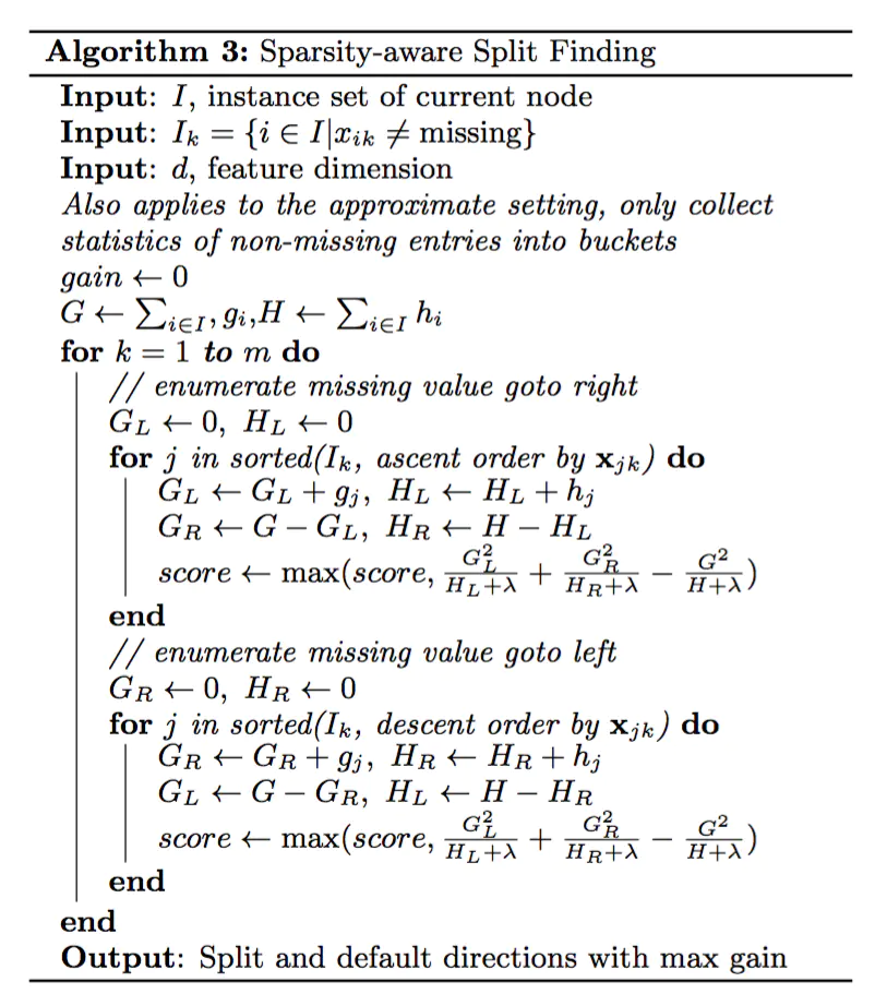
The xgboost model can handle missing values, that is, the model allows missing values to exist.
In this paper, the processing of missing values is regarded as the same as that of sparse matrix. When looking for split points, the samples with missing feature will not be traversed and counted, but only the corresponding eigenvalues on the samples with non missing feature value in this column. Through this technique, the time cost of looking for split points for sparse discrete features is reduced.
In the logical implementation, in order to ensure the completeness, the two cases of allocating the sample of missing the eigenvalue to the left leaf node and the right leaf node will be handled respectively. After calculating the gain, select the direction with large gain to split. The default direction of the branch can be specified for the missing value or the specified value, which can greatly improve the efficiency of the algorithm. If there is no missing value in the training, the If there is a missing value in the prediction, the division direction of the missing value will be automatically placed in the right subtree.
Category processing
XGBoost algorithm needs to preprocess the classification variables numerically before model training, usually using LabelEncoding or OneHotEncoding methods.
In the xgboost model, the use of onehot coding does not significantly improve the results, and sometimes it will decrease slightly. According to the data, onehot coding can not be used in the decision tree model. This operation is usually applicable to the algorithm using vector space measurement. The single hot coding of disordered classification variables can avoid the partial ordering caused by vector distance calculation. For the tree model, the It is often necessary to label the classified variables without heat alone coding.