Introduction to deep learning - from naive perceptron to neural network

Introduction: Notes for getting started with deep learning

1, Naive perceptron

1. Perceptron

Receive multiple signals and output one signal. As shown in Figure 2-1, it is a perceptron that accepts two input signals.

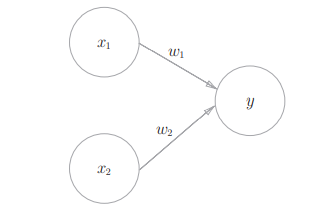Figure 2-1

X1 and X2 are input signals, y are output signals, w1 and w2 are weights. And in the picture ⚪ Represents "neuron" or "node". When the input signal is sent to the neuron, it will be multiplied by the fixed weight (w1x1, w2x2) respectively. The neuron calculates the sum of the transmitted signals and outputs 1 only when the sum exceeds a certain limit value. This is also known as "neurons are activated". Here, this limit value is called the threshold value, which is represented by a symbol θ express. Expressed by formula, as shown in Figure 2-2

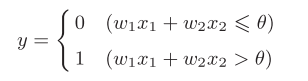Figure 2-2

2. Perceptron practice

Next, let's implement something with a perceptron and experience what a perceptron is.

2.1 the first is and gate:

And gate, i.e. 00 output 0, 01 output 0, 10 output 0, 11 output 1. X1 and X2 are input signals. We can determine W1 = 0.6 and W2 = 0.6 as long as we try a little without any skills, θ= 1 change the perceptron of Figure 2-1 into and gate. And there are countless such numerical groups that make them and gates.

2.2 NAND and or gates:

NAND gate, i.e. 00 output 1, 10 output 1, 01 output 1, 11 output 0. It also includes w1=-0.2,w2=-0.2, θ=- 0.3.

Or gate, i.e. 00 output 0, 10 output 1, 01 output 1, 11 output 1. It also includes w1=0.2,w2=0.2, θ= 0.1.

We can simplify the formula in Figure 2-2 and change it to the following
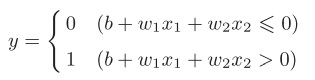Figure 2-3

We'll call the shifted b offset. In this way, we can easily implement NAND gate, NAND gate, or gate in code

import numpy as np

def AND(X):#And gate
    W = np.array([0.5, 0.5])
    b = -0.7
    tmp = np.sum(W * X) + b
    if tmp <= 0:
        return 0
    else:
        return 1
def OR(X):#Or gate
    W = np.array([0.2, 0.2])
    b = -0.1
    tmp = np.sum(W * X) + b
    if tmp <= 0:
        return 0
    else:
        return 1
def NAND(X):#NAND gate
    W = np.array([-0.2, -0.2])
    b = 0.3
    tmp = np.sum(W * X) + b
    if tmp <= 0:
        return 0
    else:
        return 1
        
x = np.array([1,1])
print(AND(x))
print(NAND(x))
print(OR(x))

2.3 we can easily get different perceptrons by changing the weight and paranoia, so let's think about how to realize XOR gate.

The XOR gate is 00 output 0, 11 output 0, 01 output 1, 10 output 1. The answer is that it cannot be realized.

Let's look at the implementation of or gate, b=-0.5,w1=1.0,w2=1.0. The perceptron expression brings the parameters into figure 2-3 to obtain the formula of figure 2-4
Figure 2-4

In this way, we can draw a straight line x1+x2=0.5 to divide two outputs, as shown in Figure 2-5 below. The output above the straight line is 1 and the output below the straight line is 0.
Figure 2-5

What is the image of the XOR gate? As shown in Figure 2-6 below, 1 is output below the curve and 0 is output above the curve.

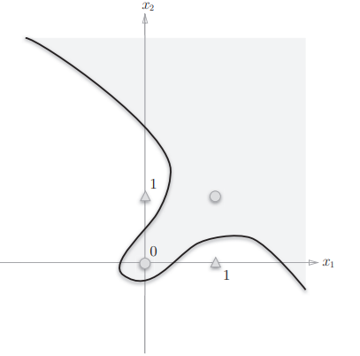Figure 2-6

3. Multilayer perceptron

Let's change our thinking and use the knowledge we have acquired. That is, use and gate, or gate and NAND gate to spell an XOR gate.

Figure 2-7

As shown below, you can draw it with a little try

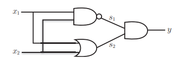Figure 2-8

In this way, we can draw the appearance of the perceptron, as shown in Figure 2-9

Figure 2-9

As shown in Figure 2-9, the multi-layer perceptron is called multi-layer perceptron. In fact, through overlay, we can realize a computer with two-layer perceptron through modular thinking. You can try to read the elements of computer system: building a modern computer from scratch, which can help us realize what the computer we learn is.

2, Neural network

1. From perceptron to neural network

Figure 3-1

As shown in the figure, it is a simple neural network, which is very similar to the perceptron. We also turn the middle layer into a hidden layer. In the previous chapter, we realized and gate, or gate, NAND gate and XOR gate with perceptron by determining the parameters. However, when the functions are more complex, it will become very difficult to find the appropriate parameters, and the emergence of neural network solves this problem well. It can find the appropriate parameters by "learning", This process of finding parameters is called "neural network learning".

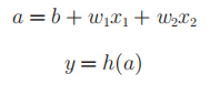
1.1. Simplification of perceptron: we can easily change the mathematical formula of perceptron to a simpler one, that is, from Figure 3-1 to figure 3-2, and then get Figure 3-3.

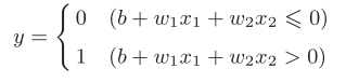Figure 3-1
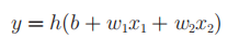Figure 3-2
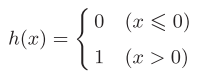Figure 3-3

2. Activate function

The h(x) function obtained from Figure 3-3 will convert the sum of input signals into output signals. This function is generally referred to as the activation function.

At this time, we can clearly show its "activation" function.

The activation function in Figure 3-3 is bounded by the threshold. Once the threshold is exceeded, the output is switched. We call this function step function. Activation function is the bridge between perceptron and neural network. We can enter the world of neural network by replacing step function with other functions.

3.sigmoid function:

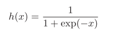Figure 3-4

exp(-x) is the - x power of e. Let's implement the sigmoid function in code and draw it for him

import numpy as np
import matplotlib.pylab as plt

def sigmoid(x): #Even if you input an array, the broadcast function
    return 1/(1+np.exp(-x))

x=np.arange(-5.0,5.0,0.1)
y=sigmoid(x)

plt.plot(x,y)
plt.ylim(-0.1,1.1) #Specify the y-axis range
plt.show()

We can see Figure 3-5

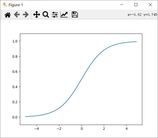Figure 3-5

​

Compare the lower step function and sigmoid function, as shown in Figure 3-6

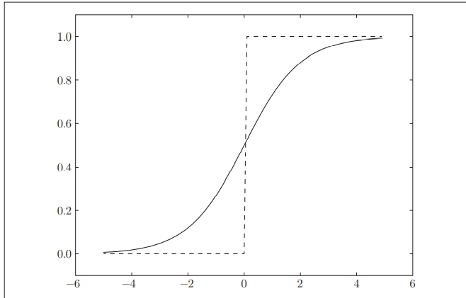
Figure 3-6

It is easy to see that sigmoid is smoother, and its smoothness will be reflected in the learning of neural network. Note that both are nonlinear functions. The activation function of neural network uses nonlinear function intelligently, because it is meaningless to use linear function neural network plus deep number. You can think about why.

3. Neural network

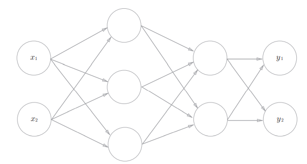
Figure 3-7

Why three layers? Because the leftmost layer x1x2 is called layer 0. Next, we use numpy to implement the three-layer neural network in Figure 3-7 below.

4.1 symbols

Figure 3-8

We join paranoia

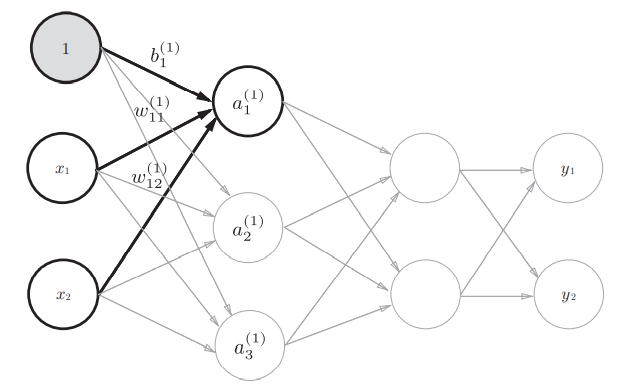
Figure 3-9

We can get the formula as shown in Figure 3-10

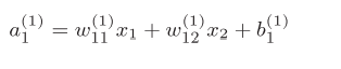
Figure 3-10

Figure 3-11

If we use a matrix, it can be expressed as A=XW+B. We assume that the parameters are arbitrary values and use code to transfer from layer 0 to layer 1

import numpy as np

def sigmoid(x):
    return 1/(1+np.exp(-x))

X = np.array([1.0,0.5])
W1 = np.array([[0.1,0.3,0.5],[0.2,0.4,0.6]])
B1 = np.array([0.1,0.2,0.3])

A1 = np.dot(X,W1)+B1
Z1 = sigmoid(A1)

print(A1)
print(Z1)

The same is true from the first layer to the second layer, and from the third layer to the fourth layer, that is, the output layer. We take the identity function as the activation function. That is, indentity_function

The code implements three-layer neural network as follows:

import numpy as np

def sigmoid(x):
    return 1/(1+np.exp(-x))

def identity_function(x):
    return x

def ini_work():
    network = {}
    network['W1'] = np.array([[0.1,0.3,0.5],[0.2,0.4,0.6]])
    network['b1'] = np.array([0.1, 0.2, 0.3])
    network['W2'] = np.array([[0.1, 0.4], [0.2, 0.5],[0.3,0.6]])
    network['b2'] = np.array([0.1, 0.2])
    network['W3'] = np.array([[0.1, 0.3], [0.2, 0.4]])
    network['b3'] = np.array([0.1, 0.2])
    return network

def forward(network,x):
    W1,W2,W3 =network['W1'],network['W2'],network['W3']
    b1,b2,b3 =network['b1'],network['b2'],network['b3']
    a1 = np.dot(x,W1)+b1
    z1 = sigmoid(a1);
    a2 = np.dot(z1,W2)+b2
    z2 = sigmoid(a2)
    a3 = np.dot(z2,W3)+b3
    y = identity_function(a3)
    return y

network = ini_work();
x = np.array([1.0,5.0])
y = forward(network,x)
print(y)

5. Design of output layer

Neural network can be used in classification and regression problems, but the activation function of the output layer needs to be changed according to the situation. Generally speaking, the regression problem uses the identity function and the classification problem uses the softmax function.

6. Identity function and softmax function

Figure 3-12 shows the softmax function

Figure 3-12

softmax function is the output function, and each neuron in the output layer is affected by all input signals. In order to prevent overflow, we improve it to figure 3-13. C 'is usually set to the maximum value of semaphore, that is, the largest one in ai.

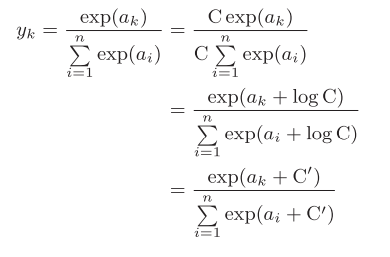
Figure 3-13

Realize it with code

import numpy as np

def softmax(a):
    c = np.max(a)
    exp_a = np.exp(a-c)
    sum_exp_a = np.sum(exp_a)
    y = exp_a/sum_exp_a
    
    return y

a = np.array([0.3,2.9,4.0])
y = softmax(a)
print(y)
print(np.sum(y))

The running result of this code is shown in Figure 3-14

Figure 3-14

As shown above, the output of the softmax function is a real number between 0.0 and 1.0. Moreover, the sum of the output values of the softmax function is 1. The output sum of 1 is an important property of softmax function. Because of this property, we can interpret the output of softmax function as "probability".

Even if the softmax function is used, the size relationship between elements will not change. This is because the exponential function (y = exp(x)) is a monotonically increasing function.

The steps of solving machine learning problems can be divided into "learning" A and "reasoning". Firstly, the model is learned in the learning stage, and then in the reasoning stage, the learned model is used to reason (classify) the unknown data. As mentioned earlier, the softmax function of the output layer is generally omitted in the reasoning stage. Softmax function is used in the output layer because it is related to the learning of neural network.

The number of neurons in the output layer is generally the same as the number of categories for classification problems.