Introduction to deep learning (2) - linear units and gradient descent

What is a linear unit:

There is a problem with perceptron. When the data set is not linearly separable, the "perceptron rule" may not converge, which means that we can never complete the training of a perceptron. In order to solve this problem, we use a derivative linear function to replace the step function of the perceptron, which is called linear element. The linear element will converge to an optimal approximation when facing the linearly inseparable data set.

For simplicity, we can set the activation function f of the linear unit as:
f ( x ) = x f(x) = x f(x)=x
After replacing the activation function in this way, the linear unit will return a real value instead of 0,1 classification. Therefore, linear units are used to solve regression problems rather than classification problems.

Linear element model:

When we talk about models, we're actually talking about algorithms that predict output based on input. For example, it can be a person's working years or his monthly salary. We can use some algorithm to predict a person's income according to his working years. For example:
y = h ( x ) = w ∗ x + b y=h(x)=w*x+b y=h(x)=w∗x+b
When x is a multidimensional vector, w should also be a multidimensional vector. At this time, the formula can be expressed as:
y = h ( x ) = w 1 ∗ x 1 + w 2 ∗ x 2 + w 3 ∗ x 3 + w 4 ∗ x 4 + b y=h(x)=w1*x1+w2*x2+w3*x3+w4*x4+b y=h(x)=w1∗x1+w2∗x2+w3∗x3+w4∗x4+b
We can also write the above formula in the form of vector:
y = h ( x ) = w T ∗ x y=h(x)=wT*x y=h(x)=wT∗x
A model that looks like this is called a linear model, because output y is a linear combination of input features * x1,x2,x3,... *

Concepts of supervised learning and unsupervised learning:

• Supervised learning: it means that in order to train a model, we need to provide a pile of training samples: each training sample includes not only the input feature * * x * * *, but also the corresponding output y***(y is also called tag, label). In other words, we need to find a lot of people. We know their characteristics (working years, industry...) and their income. Simply put, it means knowing both input and output.
• Unsupervised learning: only * * * x * * * but not * * * y * * * in the training samples of this method. The model can summarize some laws of the feature * * * x * * *, but the corresponding answer * * * y * * * cannot be known.

Realize linear unit:

There is no essential difference between the implementation of the last sensor and the linear unit, but the excitation function can be replaced by a derivative function.

from functools import reduce
import matplotlib.pyplot as plt

import numpy as np


def acti_fun(x):
    return x


class perceptron(object):
    def __init__(self, input_num):
        self.weight = [0.0] * input_num
        self.b = 0.0

    def train(self, input_vecs, labels, times, rate):  # Set the input vector, label, number of times and learning rate of training
        for i in range(times):
            for input_vec, label in zip(input_vecs, labels):
                output = acti_fun(sum(np.array(input_vec) * self.weight) + self.b)
                delta = label - output
                self.weight += rate * delta * np.array(input_vec)
                self.b += rate * delta
        return self.weight, self.b

    def predict(self, input_data):
        input_data = np.array(input_data)
        pre = []
        for data in input_data:
            pre_data = acti_fun(sum(np.array(data) * np.array(self.weight)))
            pre.append(pre_data)
        return pre


def get_training_dataset():  # Set the linear unit of data training
    input_vecs = [[5], [3], [8], [1.4], [10.1]]
    labels = [5500, 2300, 7600, 1800, 11400]
    return input_vecs, labels


def train_linear_uint():
    lu = perceptron(1)
    input_data, labels = get_training_dataset()
    lu.train(input_data, labels, 100, 0.1)
    return lu


# Draw a picture
def plot(linearUnit):
    input_data, labels = get_training_dataset()
    fig = plt.figure()
    ax = fig.add_subplot(111)
    ax.scatter(input_data, labels)
    weights = linearUnit.weight
    b = linearUnit.b
    x = range(0, 15, 1)
    y = list(map(lambda x: weights[0] * x + b, x))
    ax.plot(x, y)
    plt.show()


if __name__ == "__main__":
    # Create linear cell
    linear_unit = train_linear_uint()
    # Print weight
    print(linear_unit)
    # test
    print(linear_unit.predict([3.4]))
    print(linear_unit.predict([15]))
    print(linear_unit.predict([1.5]))
    print(linear_unit.predict([6.3]))
    plot(linear_unit)

Compare the perceptron model with the linear unit model:

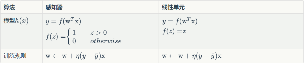
It can be seen from the above figure that the models and training rules are the same except that the activation function f is different. Then, you only need to replace the activation function of the perceptron.

Summary:

In fact, machine learning algorithm has only two parts:

• The model predicts the function h(x) of input y from the access feature X
• The parameter value corresponding to the minimum (maximum) value of the objective function is the optimal value of the parameters of the model. In many cases, we can only get the local minimum (maximum) value of the objective function, so we can only get the local optimal value of the model parameters.

Reference article:

https://www.zybuluo.com/hanbingtao/note/448086

https://blog.csdn.net/IT_job/article/details/80315364