Chapter 3 word2vec
The topic of this chapter is still the distributed representation of words. In the previous chapter, we obtained the distributed representation of words by using the counting based method. In this chapter, we will discuss the alternative method of this method, that is, the reasoning based method.
As the name suggests, the reasoning based method uses the reasoning mechanism. Of course, the reasoning mechanism here uses neural network. In this chapter, the famous word2vec will appear.
The goal of this chapter is to implement a simple word2vec. This simple word2vec prioritizes comprehensibility at the expense of processing efficiency. Therefore, we will not use it to deal with large data sets, but there is no problem with small data sets.
3.1 reasoning based methods and neural networks
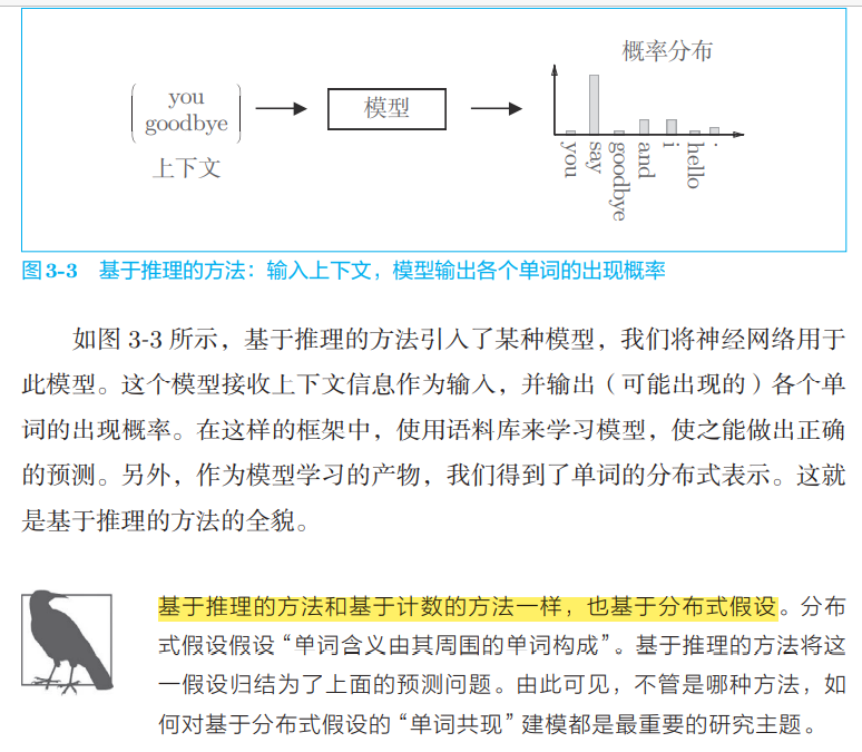
Recently, the research of using vector to represent words is in full swing. The more successful methods can be divided into two kinds: one is based on counting; The other is based on reasoning.
3.1. 1 problem of counting based method
The counting based method uses the statistical data of the whole corpus (co-occurrence matrix and PPMI, etc.) to obtain the distributed representation of words through one-time processing (SVD, etc.). The reasoning based method uses neural network, which is usually studied on mini batch data. This means that the neural network only needs to look at a part of the learning data (Mini batch) at a time and update the weight repeatedly.
The counting based method processes all learning data at one time; On the contrary, the reasoning based method uses part of the learning data to learn step by step.
3.1. 2 summary of reasoning based methods
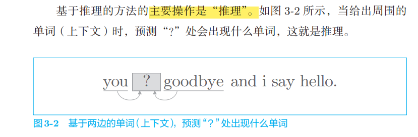
The main operation of reasoning based method is "reasoning"**
3.1. 3 word processing method in neural network
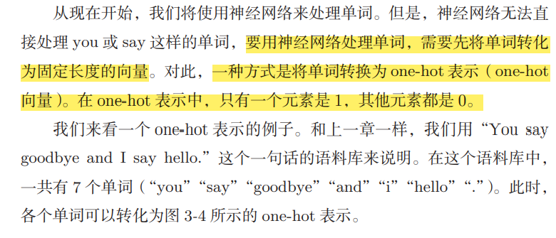
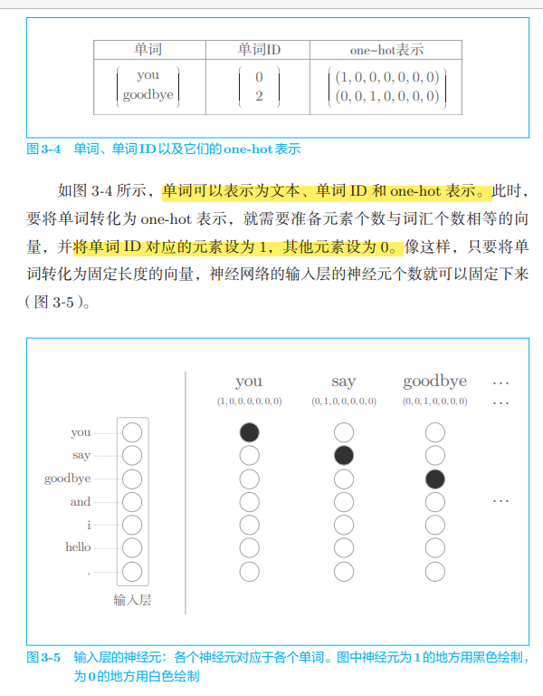
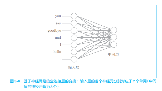
As shown in Figure 3-5, the input layer is represented by 7 neurons, corresponding to 7 words respectively (the first neuron corresponds to you and the second neuron corresponds to say)
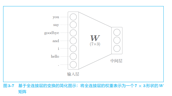
Now things are very simple. Because as long as words are represented as vectors, these vectors can be processed by various "layers" constituting neural networks. For example, for a word represented by one hot, use the full connection layer to transform it, as shown in Figure 3-6. (offset omitted)
Let's look at the code. The full connection layer transformation here can be written as follows
import numpy as np
c = np.array([[1, 0, 0, 0, 0, 0, 0]]) # input
W = np.random.randn(7, 3) # weight
h = np.dot(c, W) # Intermediate node
print(W)
print(h)

#output
[[-1.30982294  0.19485001 -0.49979452]
 [-1.77466539 -2.67810488  2.7992046 ]
 [-0.20747764 -0.68246166  0.7149981 ]
 [ 0.18558413 -0.61176428  2.25844791]
 [-0.70263837  0.63946127 -0.33276184]
 [-0.31945603  0.07161013  1.18615179]
 [ 2.01949978 -0.5961003  -1.01233551]]

[[-1.30982294  0.19485001 -0.49979452]]
class MatMul:
    def __init__(self, W):
        self.params = [W]
        self.grads = [np.zeros_like(W)]
        self.x = None

    def forward(self, x):
        W, = self.params
        out = np.dot(x, W)
        self.x = x
        return out

    def backward(self, dout):
        W, = self.params
        dx = np.dot(dout, W.T)
        dW = np.dot(self.x.T, dout)
        self.grads[0][...] = dW
        return dx
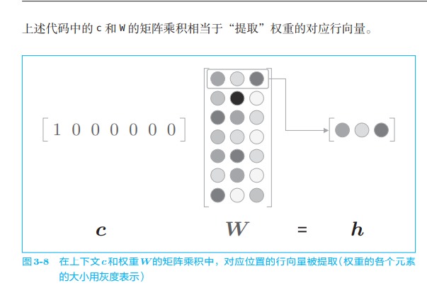
Here, it does not seem very efficient to calculate the matrix product only to extract the row vector of the weight. We will improve this in Section 4.1. In addition, the functions of the above code can also be completed by using the MatMul layer implemented in Chapter 1,
c = np.array([[1, 0, 0, 0, 0, 0, 0]])
W = np.random.randn(7, 3)
layer = MatMul(W)
h = layer.forward(c)
print(h)
# [[-0.70012195 0.25204755 -0.79774592]]
3.2 simple word2vec
Word2vec was originally used to refer to programs or tools, but with the popularity of the word, it also refers to the model of neural network in some contexts. Correctly speaking, CBOW model and skip gram model are two neural networks used in word2vec.
3.2. 1 reasoning of CBOW model
CBOW model is a neural network that predicts the target word according to the context ("target word" refers to the middle word, and the words around it are "context"). By training the CBOW model so that it can predict correctly as much as possible, we can obtain the distributed representation of words.
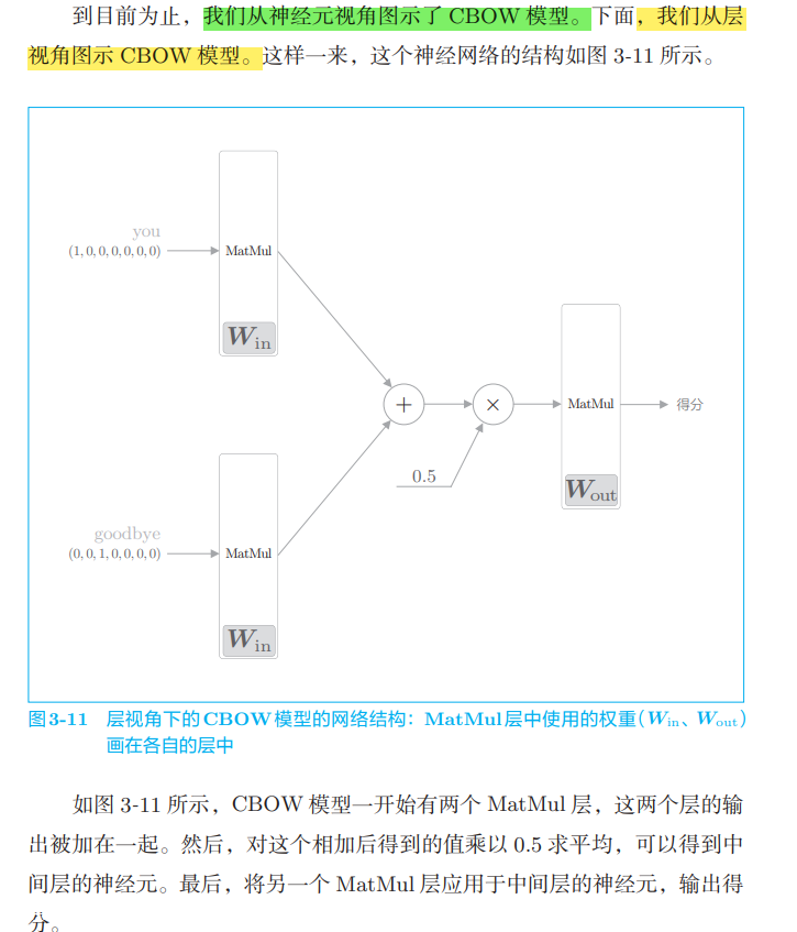
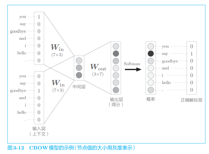
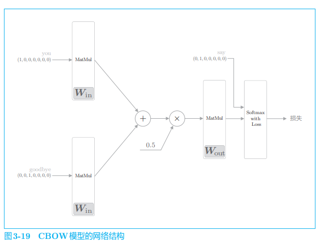
The input to the CBOW model is context. This context is represented by a list of words such as ['you', 'goodbye]. We convert it to a one hot representation so that the CBOW model can handle it. On this basis, the network of CBOW model can be drawn as shown in Figure 3-9.
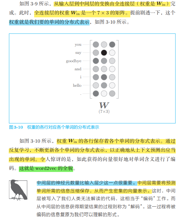
Figure 3-9 shows the network of CBOW model. It has two input layers, passing through the middle layer to the output layer. Here, the transformation from the input layer to the middle layer is completed by the same full connection layer (weight Win), and the transformation from the middle layer to the output layer is completed by another full connection layer (weight Wout).
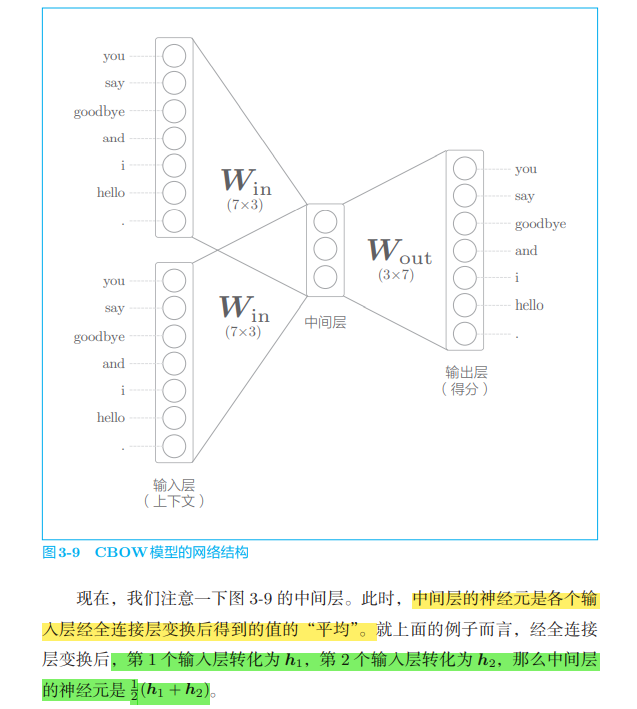
Sometimes, the neuron whose score passes through the Softmax layer is called the output layer. Here, we call the node that outputs the score as the output layer.
The processing of the full connection layer without bias is represented by the forward propagation of the MatMul layer. This layer computes the matrix product internally.
The reasoning of CBOW model is realized. The specific implementation is as follows
# coding: utf-8
import sys
sys.path.append('..')
import numpy as np
from common.layers import MatMul


# Sample context data
c0 = np.array([[1, 0, 0, 0, 0, 0, 0]])
c1 = np.array([[0, 0, 1, 0, 0, 0, 0]])

# Initialize weight
W_in = np.random.randn(7, 3)
W_out = np.random.randn(3, 7)

# Generation layer
in_layer0 = MatMul(W_in)
in_layer1 = MatMul(W_in)
out_layer = MatMul(W_out)

# Forward propagation
h0 = in_layer0.forward(c0)
h1 = in_layer1.forward(c1)
h = 0.5 * (h0 + h1)
s = out_layer.forward(h)
print(s)

# [[-0.33304998  3.19700011  1.75226542  1.36880744  1.68725368  2.38521564 0.81187955]]
The above is the reasoning process of CBOW model. The CBOW model we see here is a simple network structure without activation function. There is no difficulty except that multiple input layers share weights.
3.2. 2 CBOW model learning
The learning of CBOW model is to adjust the weight to make the prediction accurate. As a result, the weight Win (to be exact, both Win and Wout) learns the vector containing the occurrence pattern of the word. According to past experiments, the distributed representation of words obtained by CBOW model (and skip gram model), especially the distributed representation of words learned from large-scale corpora such as Wikipedia, has many cases that accord with our intuition in word meaning and grammar
CBOW model only learns the occurrence patterns of words in the corpus. If the corpus is different, the distributed representation of the learned words is also different. For example, the distributed representation of words obtained by using only "Sports" related articles will be very different from that obtained by using only "music" related articles.
3.2. 3 weight and distributed representation of word2vec
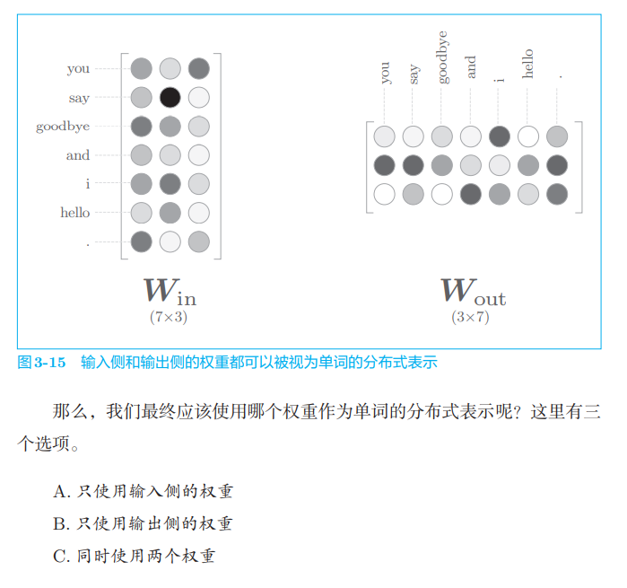
In terms of word2vec (especially skip gram model), the most popular is scheme A. Following this idea, we also use Win as the distributed representation of words
3.3 preparation of learning data
Before starting the learning of word2vec, let's prepare the data for learning. Here we still say "You say goodbye and I say hello." This one sentence corpus is illustrated as an example.
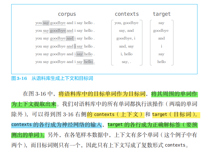
3.3. 1 context and target words
The input of the neural network used in word2vec is context, and its correct unlabeling is the word surrounded by these contexts, that is, the target word.
def preprocess(text):
    text = text.lower()
    text = text.replace('.', ' .')
    words = text.split(' ')

    word_to_id = {}
    id_to_word = {}
    for word in words:
        if word not in word_to_id:
            new_id = len(word_to_id)
            word_to_id[word] = new_id
            id_to_word[new_id] = word

    corpus = np.array([word_to_id[w] for w in words])

    return corpus, word_to_id, id_to_word
We implement the function of generating context and target words from corpus. Before that, let's review the content of the previous chapter. First, the text of the corpus is transformed into word ID.
import sys
sys.path.append('..')
from common.util import preprocess
text = 'You say goodbye and I say hello.'
corpus, word_to_id, id_to_word = preprocess(text)
print(corpus)
# [0 1 2 3 4 1 5 6]
print(id_to_word)
# {0: 'you', 1: 'say', 2: 'goodbye', 3: 'and', 4: 'i', 5: 'hello', 6: '.'}
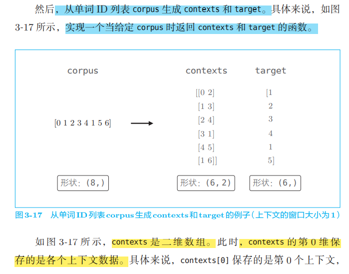
Create function to generate context and target words_ contexts_ target(corpus, window_size)
def create_contexts_target(corpus, window_size=1):
    '''Generate context and target words

    :param corpus: Corpus (words) ID (list)
    :param window_size: Window size (when the window size is 1, 1 word on the left and right is the context)
    :return:
    '''
    target = corpus[window_size:-window_size]
    contexts = []

    for idx in range(window_size, len(corpus)-window_size):
        cs = []
        for t in range(-window_size, window_size + 1):
            if t == 0:
                continue
            cs.append(corpus[idx + t])
        contexts.append(cs)

    return np.array(contexts), np.array(target)
Following the implementation just now, the code is as follows.
contexts, target = create_contexts_target(corpus, window_size=1)
print(contexts)
# [[0 2]
# [1 3]
# [2 4]
# [3 1]
# [4 5]
# [1 6]]
print(target)
# [1 2 3 4 1 5]
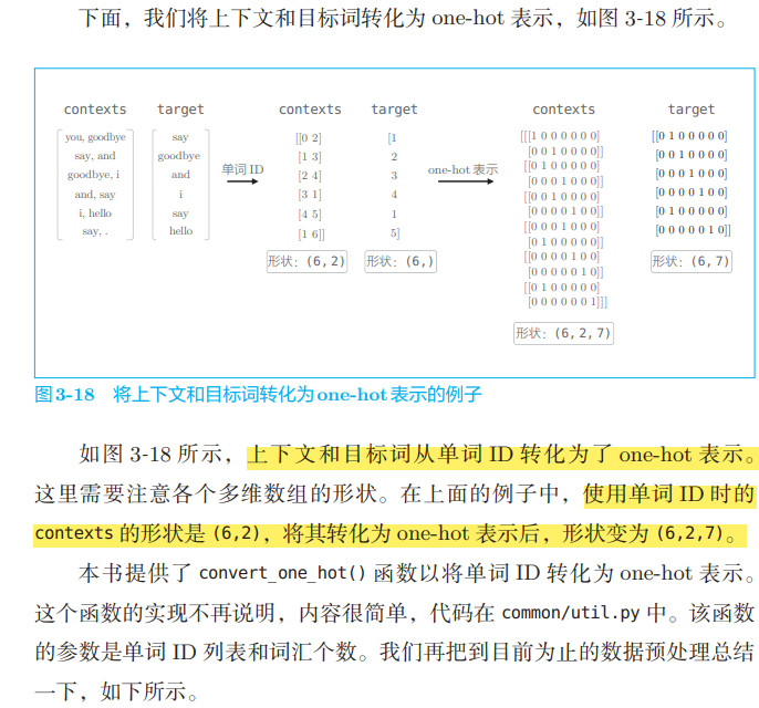
3.3. 2 convert to one hot representation
def convert_one_hot(corpus, vocab_size):
    '''Convert to one-hot express

    :param corpus: word ID List (one or two dimensional) NumPy Array)
    :param vocab_size: Number of words
    :return: one-hot Representation (2D or 3D) NumPy Array)
    '''
    N = corpus.shape[0]

    if corpus.ndim == 1:
        one_hot = np.zeros((N, vocab_size), dtype=np.int32)
        for idx, word_id in enumerate(corpus):
            one_hot[idx, word_id] = 1

    elif corpus.ndim == 2:
        C = corpus.shape[1]
        one_hot = np.zeros((N, C, vocab_size), dtype=np.int32)
        for idx_0, word_ids in enumerate(corpus):
            for idx_1, word_id in enumerate(word_ids):
                one_hot[idx_0, idx_1, word_id] = 1

    return one_hot
Implementation code: the preparation of learning data is completed
text = 'You say goodbye and I say hello.'

corpus, word_to_id, id_to_word = preprocess(text)

contexts, target = create_contexts_target(corpus, window_size=1)

vocab_size = len(word_to_id)

target = convert_one_hot(target, vocab_size)

contexts = convert_one_hot(contexts, vocab_size)
contexts

#Output contexts
array([[[1, 0, 0, 0, 0, 0, 0],
        [0, 0, 1, 0, 0, 0, 0]],

       [[0, 1, 0, 0, 0, 0, 0],
        [0, 0, 0, 1, 0, 0, 0]],

       [[0, 0, 1, 0, 0, 0, 0],
        [0, 0, 0, 0, 1, 0, 0]],

       [[0, 0, 0, 1, 0, 0, 0],
        [0, 1, 0, 0, 0, 0, 0]],

       [[0, 0, 0, 0, 1, 0, 0],
        [0, 0, 0, 0, 0, 1, 0]],

       [[0, 1, 0, 0, 0, 0, 0],
        [0, 0, 0, 0, 0, 0, 1]]])
3.4 implementation of cbow model
class SimpleCBOW:
def __init__(self, vocab_size, hidden_size):
V, H = vocab_size, hidden_size #Vocabulary number vocab_size, number of neurons in the middle layer hidden_size
# Initialize the weights and initialize the two weights with some small random values. astype('f ') initialization will use 32-bit floating-point numbers.
W_in = 0.01 * np.random.randn(V, H).astype('f')
W_out = 0.01 * np.random.randn(H, V).astype('f')
# Generation layer
#Generate two input side MatMul layers, one output side MatMul layer, and one Softmax with Loss layer.
self.in_layer0 = MatMul(W_in)
self.in_layer1 = MatMul(W_in)
self.out_layer = MatMul(W_out)
self.loss_layer = SoftmaxWithLoss()
# Organize all weights and gradients into a list
layers = [self.in_layer0, self.in_layer1, self.out_layer]
self.params, self.grads = [], []
for layer in layers:
self.params += layer.params
self.grads += layer.grads
# Set the distributed representation of the word as a member variable
self.word_vecs = W_in
#Forward propagation function of neural networks
def forward(self, contexts, target):
h0 = self.in_layer0.forward(contexts[:, 0])
h1 = self.in_layer1.forward(contexts[:, 1])
h = (h0 + h1) * 0.5
score = self.out_layer.forward(h)
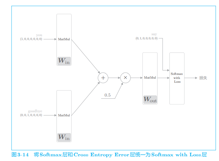
loss = self.loss_layer.forward(score, target)
return loss
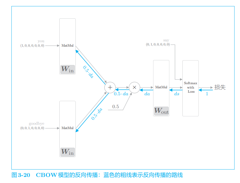
def backward(self, dout=1):
ds = self.loss_layer.backward(dout)
da = self.out_layer.backward(ds)
da *= 0.5
self.in_layer1.backward(da)
self.in_layer0.backward(da)
return None
Here, the number of MatMul layers used to process the input side context is the same as the number of words in the context (two in this example). In addition, we use the same weight to initialize the MatMul layer.
Finally, the weight parameters and gradients used in the neural network are saved in the list type member variables params and grads respectively.
Here, multiple layers share the same weight. Therefore, there are multiple identical weights in the params list. However, when there are multiple identical weights in the params list, the operation of optimizers such as Adam and Momentum will become unexpected (at least in terms of our code). For this reason, inside the Trainer class, a simple de duplication operation will be performed when updating parameters. For this point, the description is omitted here. Interested readers can refer to common / Trainer Remove of PY_ duplicate(params, grads)
Here, we assume that the parameter contexts is a three-dimensional NumPy array, that is, the shape in the example (6,2,7) in Figure 3-18 in the previous section, where the number of elements in dimension 0 is the number of mini batch, the number of elements in dimension 1 is the window size of the context, and the second dimension represents the one hot vector. In addition, the target is a two-dimensional shape such as (6,7).
So far, the implementation of back propagation is over. We have saved the gradient of each weight parameter in the member variable grads. Therefore, by calling the forward() function first and then the backward() function, the grads in the grads list is updated. Next, let's continue to look at the learning of the simplecrow class
Realization of learning
The learning of CBOW model is exactly the same as that of general neural network. First, prepare the learning data for the neural network. Then, calculate the gradient and gradually update the weight parameters. Here, we use the Trainer class introduced in Chapter 1 to perform the learning process,
import sys
sys.path.append('..')  # Settings for importing files from the parent directory
from common.trainer import Trainer
from common.optimizer import Adam
from simple_cbow import SimpleCBOW
from common.util import preprocess, create_contexts_target, convert_one_hot


window_size = 1
hidden_size = 5
batch_size = 3
max_epoch = 1000

text = 'You say goodbye and I say hello.'
corpus, word_to_id, id_to_word = preprocess(text)

vocab_size = len(word_to_id)
contexts, target = create_contexts_target(corpus, window_size)
target = convert_one_hot(target, vocab_size)
contexts = convert_one_hot(contexts, vocab_size)

model = SimpleCBOW(vocab_size, hidden_size)
optimizer = Adam()
trainer = Trainer(model, optimizer)

trainer.fit(contexts, target, max_epoch, batch_size)
trainer.plot()

word_vecs = model.word_vecs  #The weight of the MatMul layer on the input side has been assigned to the member variable word_vecs
for word_id, word in id_to_word.items():
    print(word, word_vecs[word_id])
you [ 1.1550112  1.2552509 -1.1116056  1.1482503 -1.2046812]
say [-1.2141827  -1.2367412   1.2163384  -1.2366292   0.67279905]
goodbye [ 0.7116186   0.55987084 -0.8319744   0.749239   -0.8436555 ]
and [-0.94652086 -0.8535852   0.55927175 -0.6934891   2.0411916 ]
i [ 0.7177702  0.5699475 -0.8368816  0.7513028 -0.8419596]
hello [ 1.1411363  1.2600429 -1.105042   1.1401148 -1.2044929]
. [-1.1948084 -1.2921802  1.4119368 -1.345656  -1.5299033]
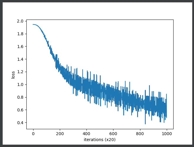
Unfortunately, the small corpus used here does not give good results. Of course, the main reason is that the corpus is too small. If we change to a larger and more practical corpus, we believe we will get better results. However, there will be new problems in processing speed, because there are several problems in processing efficiency in the implementation of the current CBOW model. In the next chapter, we will improve this simple CBOW model and implement a "real" CBOW model.
3.5 additional notes to word2vec
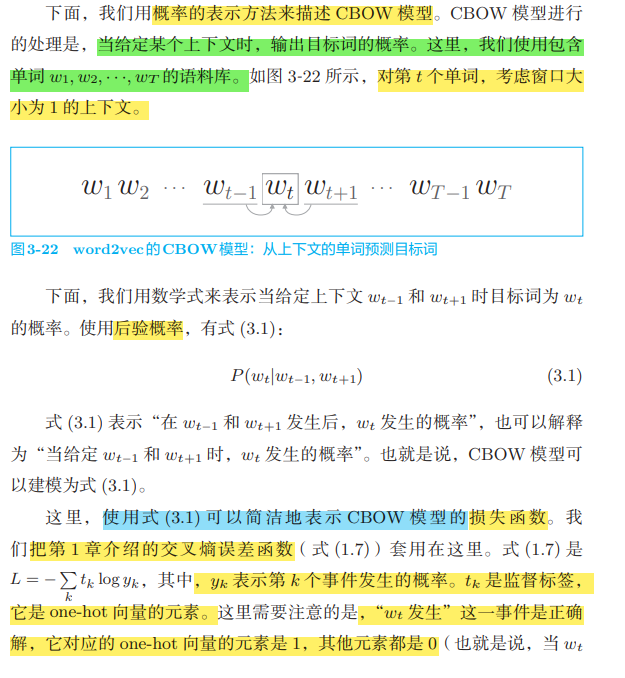
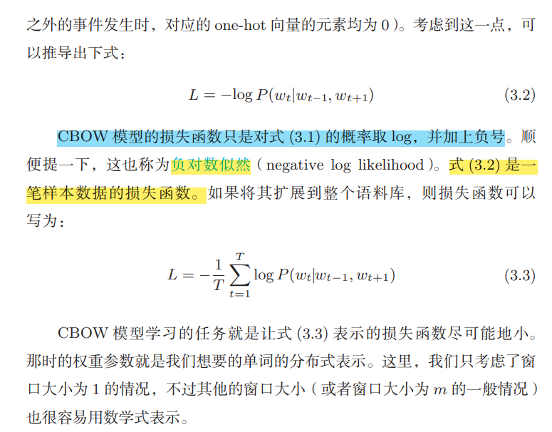
3.5. 1 CBOW model and probability
In this book, the probability is recorded as P(·), for example, the probability of event a is recorded as P(A). The joint probability is marked as * * P(A, B), indicating the probability that event a and event B occur at the same time. A posteriori probability is recorded as P(A|B) * *, which literally means "probability after the event". From another point of view, it can also be interpreted as "the probability that event a occurs when event B (information) is given".
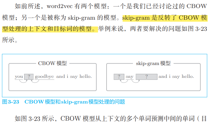
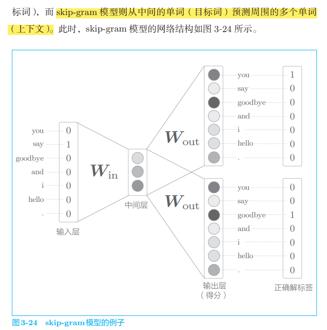
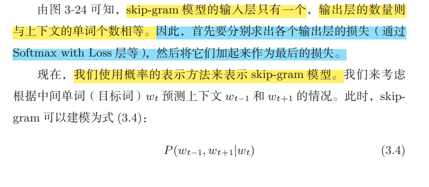
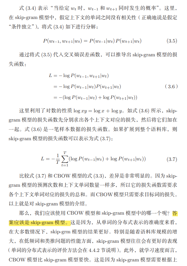
3.5. 2 skip gram model
import sys
sys.path.append('..')
import numpy as np
from common.layers import MatMul, SoftmaxWithLoss


class SimpleSkipGram:
    def __init__(self, vocab_size, hidden_size):
        V, H = vocab_size, hidden_size

        # Initialize weight
        W_in = 0.01 * np.random.randn(V, H).astype('f')
        W_out = 0.01 * np.random.randn(H, V).astype('f')

        # Generation layer
        self.in_layer = MatMul(W_in)
        self.out_layer = MatMul(W_out)
        self.loss_layer1 = SoftmaxWithLoss()
        self.loss_layer2 = SoftmaxWithLoss()

        # Organize all weights and gradients into a list
        layers = [self.in_layer, self.out_layer]
        self.params, self.grads = [], []
        for layer in layers:
            self.params += layer.params
            self.grads += layer.grads

        # Set the distributed representation of the word as a member variable
        self.word_vecs = W_in

    def forward(self, contexts, target):
        h = self.in_layer.forward(target)
        s = self.out_layer.forward(h)
        l1 = self.loss_layer1.forward(s, contexts[:, 0])
        l2 = self.loss_layer2.forward(s, contexts[:, 1])
        loss = l1 + l2
        return loss

    def backward(self, dout=1):
        dl1 = self.loss_layer1.backward(dout)
        dl2 = self.loss_layer2.backward(dout)
        ds = dl1 + dl2
        dh = self.out_layer.backward(ds)
        self.in_layer.backward(dh)
        return None
class MatMul:
    def __init__(self, W):
        self.params = [W]
        self.grads = [np.zeros_like(W)]
        self.x = None

    def forward(self, x):
        W, = self.params
        out = np.dot(x, W)
        self.x = x
        return out

    def backward(self, dout):
        W, = self.params
        dx = np.dot(dout, W.T)
        dW = np.dot(self.x.T, dout)
        self.grads[0][...] = dW
        return dx

class SoftmaxWithLoss:
    def __init__(self):
        self.params, self.grads = [], []
        self.y = None  # Output of softmax
        self.t = None  # Supervision label

    def forward(self, x, t):
        self.t = t
        self.y = softmax(x)

        # When the supervised tag is a one hot vector, it is converted to the index of the correct solution tag
        if self.t.size == self.y.size:
            self.t = self.t.argmax(axis=1)

        loss = cross_entropy_error(self.y, self.t)
        return loss

    def backward(self, dout=1):
        batch_size = self.t.shape[0]

        dx = self.y.copy()
        dx[np.arange(batch_size), self.t] -= 1
        dx *= dout
        dx = dx / batch_size

        return dx
3.5. 3 counting based and reasoning based
In addition, after word2vec, researchers proposed GloVe method [27]. GloVe method combines reasoning based method and counting based method. The idea of this method is to incorporate the statistical data of the whole corpus into the loss function for mini batch learning (please refer to paper [27]). Accordingly, the two methodologies were successfully integrated.
3.6 summary
In this chapter, we explain the CBOW model of word2vec in detail and implement it. CBOW model is basically a two-layer neural network with very simple structure. We constructed CBOW model using MatMul layer and Softmax with Loss layer, and confirmed its learning process with a small-scale corpus. Unfortunately, there are still some problems in the processing efficiency of CBOW model at this stage. However, after understanding the CBOW model in this chapter, it is one step away from the real word2vec. In the next chapter, we will improve the CBOW model.
What is learned in this chapter
- The reasoning based method aims at prediction and obtains the distributed representation of words as by-products
- word2vec is a reasoning based method, which is composed of a simple two-layer neural network
- word2vec has skip gram model and CBOW model
- CBOW model predicts one word (target word) from multiple words (context)
- The skip gram model in turn predicts multiple words (context) from one word (target word)
- Because word2vec can carry out incremental learning of weights, it can efficiently update or add the distributed representation of words